
 Open Access
Constraint Audited Receding Horizon Dispatch for Curtailment Recovery in Export Capped Utility Scale Photovoltaic Plants With Battery Energy Storage

 View Full Article|
 Download PDF
Abstract:
Hard point-of-interconnection (POI) export limits can strand otherwise-available photovoltaic (PV) energy unless battery storage is dispatched with sufficient anticipation and under physically consistent constraints. This study evaluates a constraint-audited receding-horizon dispatch framework for curtailment recovery at an anonymized 230 MW utility-scale PV plant with a modeled 195.5 MW export cap and a nominal 30 MW/140 MWh battery energy storage system (BESS). The mixed-integer model predictive controller enforces BESS power and energy limits, charge–discharge exclusivity, no grid charging, forecast-dependent discharge headroom, first-action receding-horizon execution, and a common 50%-to-50% terminal-energy protocol. Twelve rolling monthly folds from September 2024 to August 2025 are evaluated against cap-only operation and a protocol-matched perfect-information Oracle. Cap-only operation curtails 26,279 MWh (4.9872% of evaluated PV energy). A transparent 72 h Diurnal model predictive control (MPC) reduces curtailment to 11,719.454 MWh, recovers 14,559.546 MWh, and closes 98.450% of the modeled cap-only-to-Oracle recoverable-energy opportunity; the matched Oracle curtails 11,490.175 MWh. All 3 h closed-loop trajectories satisfy the modeled export cap, BESS limits, terminal equality, charge–discharge exclusivity, discharge-headroom rule, and no-grid-import condition. A matched information-sensitivity analysis then compares History-CatBoost and Weather-CatBoost under the same controller. Weather-CatBoost lowers daylight mean absolute error (MAE) by 2.225 MW at 24 h and 1.175 MW at 72 h relative to History-CatBoost, while annual curtailment is 288.601 MWh higher at 24 h and 99.699 MWh lower at 72 h; the monthly block-bootstrap intervals include zero in both cases. Histogram gradient boosting (HGB) robustness and BESS-sensitivity results further show that the incremental control value of weather information is model- and configuration-dependent. Under the tested plant, cap, BESS, 3 h resolution, horizon, and terminal protocol, physically constrained anticipatory dispatch captures most of the modeled recoverable curtailed energy, leaving comparatively limited residual opportunity for additional forecast sophistication.
1. Introduction
Utility-scale photovoltaic (PV) plants can produce more active power than a grid connection is permitted to export. Such a point-of-interconnection (POI) limit can arise from an interconnection agreement, equipment rating, congestion-management requirement, or protection constraint. When available generation exceeds that boundary, the excess must be curtailed unless another resource can absorb it. Curtailment under an undersized or constrained POI is therefore a direct energy-routing problem, and recent studies of constrained and hybrid renewable plants show that the magnitude of this loss depends on both the connection boundary and the temporal resolution at which it is evaluated [1], [2], [3], [4].
A co-located battery energy storage system (BESS) can recover part of this otherwise-lost energy by charging during above-cap PV periods and discharging later when export headroom becomes available. The useful role of storage in this setting is not generic arbitrage: it is temporal routing of renewable energy through a constrained interface. Whether that routing succeeds depends on BESS power, usable energy, efficiency, state of charge (SOC), the timing of cap-binding events, and the controller’s ability to preserve headroom before future surplus arrives.
Model predictive control (MPC) is an established framework for this class of constrained intertemporal problem. It can schedule charging, discharging, stored energy, export, and curtailment over a finite horizon while applying only the first action before the optimization is repeated [5], [6], [7]. Mixed-integer linear programming (MILP) is likewise well established for enforcing logical operating modes such as charge–discharge exclusivity. Here, MILP–MPC is used as the optimization engine within a matched closed-loop protocol that attributes curtailment recovery among storage, causal look-ahead, forecast information, and perfect information while holding the physical envelope and terminal-energy treatment fixed.
Fair benchmarking is particularly important for storage. A controller that finishes an evaluation period with less stored energy can appear to have exported or recovered more energy simply because it depleted the battery. Conversely, a perfect-information benchmark can become artificially advantaged if future realized PV is allowed to alter terminal preparation in a way unavailable to causal controllers. A defensible comparison therefore requires common initial and final stored energy, a causal terminal-feasibility treatment shared across methods, matched plant constraints, and a perfect-information benchmark that differs only in the information intentionally assigned to it.
This leads to a useful performance hierarchy. Cap-only operation measures the renewable-energy loss imposed by the export boundary without storage. A causal forecast-driven MPC measures how much of that loss can be recovered through anticipatory constrained dispatch. A protocol-matched perfect-information Oracle then defines the modeled recoverable-energy opportunity under the same BESS and terminal conditions. The fraction of the cap-only-to-Oracle opportunity already captured by a simple causal controller reveals how much room remains for more sophisticated prediction. This interpretation is complementary to forecast-centric and decision-focused work showing that lower prediction error does not necessarily produce better downstream decisions [8], [9], [10], [11], [12], [13].
Previous PV–BESS studies address complementary control questions. Forecast-based strategies for PV battery systems examine how prediction affects energy use and operating schedules [14], [15]. Mixed-integer MPC has been applied to PV plants with non-ideal storage [6]; stochastic MPC and multiobjective PV–BESS scheduling also consider prediction uncertainty and competing operating objectives [7], [16]. Decision-focused PV–battery scheduling evaluates the effect of prediction on the resulting dispatch [12]. The present formulation minimizes export-cap curtailment with a subordinate throughput penalty, explicit PV-only charging, a forecast-based discharge-headroom restriction, and a common monthly terminal-energy condition. Diurnal, history-based, weather-informed, and perfect-PV information enter the same finite-horizon MILP–MPC, followed by an audit of the executed three-hour trajectories. These common operating and terminal rules provide the basis for comparing the information streams.
Probabilistic PV–BESS control addresses a related but distinct methodological question: how forecast uncertainty should be represented and propagated through stochastic or scenario-based scheduling. Such approaches may use quantile forecasts, calibrated prediction intervals, shared scenario decisions, or risk-sensitive headroom management. The present study instead asks how curtailment recovery should be attributed when the physical envelope, terminal-energy basis, and execution protocol are held fixed. Its forecasting branches therefore serve as controlled information inputs to a deterministic receding-horizon benchmark rather than as a probabilistic-control architecture. The principal comparisons concern horizon length, protocol-matched perfect-information opportunity, terminal fairness, and realized physical integrity, with operational numerical weather prediction (NWP) evaluated as an incremental information sensitivity.
Forecast sophistication is evaluated as a secondary information-sensitivity layer after the physical control benchmark is established. A transparent Diurnal reference, a matched History-CatBoost residual forecast, and a Weather-CatBoost residual forecast that additionally receives operational NWP are frozen before closed-loop evaluation. The learned branches use the same chronological support, model family, tuning budget, weighting, residual structure, shrinkage, and fallback rules, so their difference isolates the incremental use of NWP as far as the available data permit.
The contribution of this study is an integrated control-evaluation and attribution protocol for determining how much export-cap curtailment is recoverable by causal storage dispatch and how much modeled opportunity remains for additional information. First, a hard POI limit is combined with physically constrained BESS dispatch, charge–discharge exclusivity, no grid charging, forecast-dependent discharge headroom, first-action receding-horizon execution, and realized-trajectory auditing. Second, a common 50%-to-50% terminal-energy protocol with causal terminal preparation places the causal controllers and protocol-matched Oracle on the same stored-energy basis. Third, the Cap-only–causal MPC–Oracle hierarchy separates curtailment recovery attributable to storage and anticipatory control from the residual opportunity available to additional information. Fourth, forecast streams are generated chronologically and frozen before control evaluation, after which monthly paired inference, model-family robustness, and independent BESS power and energy sensitivities quantify the remaining information effect.
Section 2 describes the PV–BESS model, receding-horizon controller, terminal protocol, forecasting inputs, and evaluation methods. Section 3 reports the control, forecast-information, and robustness results. Sections 4–6 present the discussion, limitations, and conclusions.
2. Methodology
The case study uses measured active-power records from an anonymized 230 MW grid-connected PV plant. The plant identity and raw measurements are withheld due to contractual confidentiality. The research export boundary is represented as
where, $\alpha$ denotes the export-cap fraction (0.85), and $P^{\text {rated }}$ denotes the rated PV plant capacity (230 MW). The 195.5 MW value is a modeling boundary for the present experiment and is not presented as a confirmed plant operating limit. The hourly records were timestamped in plant local standard time (Coordinated Universal Time (UTC)+4), quality controlled, and converted to UTC. Hourly power values were then averaged over nonoverlapping intervals [$t$, $t$ + 3 h) to form the common three-hour PV series. This interval matches the three-hour NWP forecast lead spacing and defines the duration of each scheduled battery action. The export cap is applied to the resulting interval-average power. Accordingly, curtailment energy and constraint compliance are evaluated consistently on the three-hour forecast–dispatch grid adopted in this study. Two isolated missing hours were interpolated, one duplicated timestamp was resolved, and observations above the declared 230 MW rating were clipped before aggregation. The common closed-loop evaluation covers twelve monthly folds from September 2024 through August 2025 and contains 526,931 MWh of measured PV energy.
The nominal BESS has symmetric 30 MW charging and discharging limits, 140 MWh nameplate energy, charge and discharge efficiencies of 0.95, and a 10–90% SOC operating range. Initial and final stored energy are both fixed at 50% of nameplate energy, i.e., 70 MWh in the nominal case. Grid charging is not allowed; the battery is used as a PV-curtailment-recovery resource.
Without storage, realized export and curtailment at interval $t$ are
For a 3 h interval $\Delta t$, total cap-only curtailed energy is
For any storage controller $m$, the reduction in modeled curtailed PV energy relative to cap-only operation is
Let $O$ denote the protocol-matched perfect-information Oracle. The modeled recoverable-energy opportunity is
and the Oracle-gap closure of controller $m$ is
where, $O$ denotes the receding-horizon MILP–MPC supplied with the realized future PV sequence outside the common terminal-steering window. During terminal preparation it receives the same Diurnal forecast as every other controller. All methods share the BESS and POI limits, the monthly initial and final energy, and the same first-action execution rule. The model represents PV generation, BESS operation, and grid export at the POI, without a separately modeled local electrical load. Thus $R_O$ is the opportunity represented by this finite-horizon information comparator, and $C_m$ measures closure relative to that comparator. No full-period global optimum is implied.
PV-only charging allows the battery to absorb both above-cap surplus and PV generation that could otherwise have been exported. Accordingly, $R_m$ measures avoided modeled curtailment, while the net export change is $E_g^m-E_g^{\text {cap}}$. With equal initial and final battery energy, charging and discharge losses can make these two quantities different. The control results report both curtailed and exported energy. The fixed physical, forecasting, and control configurations are summarized in Table 1.
Item | Value | Role in the Comparison |
|---|---|---|
PV and export boundary | 230 MW; 195.5 MW cap | Fixed plant-side active-power envelope |
Nominal BESS | 30 MW/140 MWh | Symmetric charge/discharge power limits |
Efficiency and SOC range | \(\eta_c\) = \(\eta_d\) = 0.95; 10–90% | Stored-energy range 14–126 MWh |
Initial and final SOC | 50% and 50% | Exactly 70 MWh at every nominal fold start and fold end |
Time step and horizons | 3 h; 24 h and 72 h | 8 and 24 MPC steps, respectively |
Charging source | PV only | Grid charging prohibited |
Diurnal | Same valid-time slot 24 h earlier | Transparent causal reference |
History-CatBoost | PV history and calendar variables | Learned no-weather information layer |
Weather-CatBoost | History features plus operational NWP | Incremental weather-information layer |
Oracle | Realized PV outside terminal window | Protocol-matched perfect-information benchmark |
Terminal window | 168 h prebuffer + 24 h endgame | Common causal terminal steering for every method |
At decision time $t$, the controller receives a PV trajectory over the active horizon. The first entry is the measured PV power and is therefore common to all methods; future entries come from the information stream under evaluation:
For compactness, the decision-time index $t$ is omitted below and $\tilde{P}_{k \mid t}^{\text {pv }}$ is written as $\tilde{P}_k^{\text {pv }}$. Let $\mathcal{K}=\{0, \ldots, H-1\}$. The decision variables are charging power $P_k^{\text {ch}}$, discharging power $P_k^{\text {dis}}$, grid export $P_k^g$, curtailed PV power $P_k^{\text {curt }}$, stored energy $E_k$, binary charge-mode variable $z_k$, and nonnegative terminal-deviation variables $\xi^{+}$ and $\xi^{-}$. The stored-energy limits and target are
$E_B$ is the BESS nameplate energy capacity (140 MWh). Forecast-dependent export headroom is
which is evaluated from the PV input before each optimization. The constraint $P_k^{\text {dis}} \leq h_k$ is an additional, conservative dispatch rule: it reserves forecast PV export headroom by withholding discharge when forecast PV reaches the cap. Grid export remains governed by the power balance and POI constraint, Eqs. (12) and (13). A different feasible allocation of charging and curtailment could satisfy those equations without satisfying this additional discharge rule. The controller retains the restriction for every compared information stream.
The receding-horizon MILP is
where, $E_t^{\text {meas }}$ denotes the measured battery stored energy at decision time $t$, while $P^{{\text {ch}}, \max }$ and $P^{{\text {dis}}, \max }$ denote the maximum charging and discharging powers, respectively. The weights are $w_{\text {curt }}$ = 1000, $w_{\text {thr }}$ = 1, and $w_{\text {term }}$ = 50 for every method and both horizons. The curtailed-energy weight gives priority to PV utilization; the lower throughput weight discourages unnecessary cycling, and the terminal weight penalizes deviation from the target energy at the end of an ordinary prediction horizon. The chosen values define a curtailment-prioritized dispatch and do not constitute a battery-degradation or economic calibration. Charging cannot exceed the modeled available PV, and grid charging is excluded by the nonnegative-export constraint, power balance, and charge–discharge exclusivity. The power balance permits diversion of exportable PV into the battery. At $k$ = 0, the common PV input and the associated headroom are used to form the first scheduled action.
All MILPs are solved through scipy.optimize.milp with the HiGHS backend. The nominal horizons contain 8 or 24 three-hour intervals, corresponding to 24 h and 72 h. In an ordinary solve, Eq. (22) and the objective’s terminal-deviation term permit a soft endpoint target at the prediction horizon. If the actual monthly fold endpoint falls within the nominal horizon, the horizon is shortened to that boundary and the exact terminal condition
is imposed. At that boundary the terminal-deviation variables are zero, so the soft penalty does not alter the fixed endpoint. The common steering policy described below supports reachability of this equality across the compared controllers.
Only the first optimized charging and discharging commands are executed. Stored energy is then updated using the battery model and the realized action before the horizon advances and the optimization is solved again. This first-action implementation distinguishes the results from open-loop schedule evaluation and ensures that forecast errors affect the state trajectory only through actions actually taken.
Optimization constraints alone are not treated as sufficient evidence of physical validity. The realized closed-loop trajectories are independently checked for POI-cap violation, SOC lower- or upper-bound violation, simultaneous charging and discharging, grid import, discharge beyond available headroom, battery-induced curtailment, compliance with the steering floor, solver completion, and exact terminal energy. The audit is performed after execution and state updating so that post-optimization inconsistencies cannot be hidden by solver feasibility alone.
Each monthly fold starts at 50% SOC and must finish at the same level, corresponding to 70 MWh for the nominal BESS. This common endpoint prevents one controller from obtaining an apparent energy advantage by leaving less energy in storage. Each fold is evaluated with its own initial and final energy condition.
Terminal preparation occupies the last 192 h of each fold: a 168 h prebuffer and a 24 h endgame. During the prebuffer, the lower permitted energy floor increases in seven 8 MWh increments at 19:00 plant-local time. The floor reaches the 70 MWh target at the start of the endgame and is combined with backward-reachable energy limits to preserve the remaining terminal path. When the actual fold endpoint enters the MPC horizon, the controller applies Eq. (24) exactly. Ordinary horizons use the soft terminal-deviation penalty in Eq. (11).
During the prebuffer and endgame, Diurnal, History-CatBoost, Weather-CatBoost, and Oracle use the same Diurnal forecasting rule for terminal steering while retaining the common current PV input. Elsewhere, each uses its designated forecast sequence; the Oracle alone receives realized future PV. This common terminal policy holds the end-of-fold preparation and target energy fixed across the information comparisons. This shared steering rule was adopted to reduce forecast-dependent differences in terminal preparation and preserve comparability across controllers.
The comparison is interpreted in the following order. Cap-only operation establishes the curtailment burden created by the POI limit without storage. Diurnal MPC establishes the recovery attainable with a transparent causal look-ahead signal and the same BESS. History-CatBoost tests whether nonlinear residual learning from PV history and calendar information changes that recovery. Weather-CatBoost adds operational NWP under the matched forecasting design. Finally, the protocol-matched Oracle provides a perfect-PV information reference within the same plant, BESS, finite horizon, terminal, and execution rules.
This hierarchy avoids crediting an advanced forecast with curtailment reduction that is principally attributable to the existence of storage or to anticipatory control itself. It also makes the remaining Oracle gap operationally interpretable: when a simple causal controller already closes almost all of the modeled recoverable opportunity, forecast improvement has little objective space in which to create an additional gain.
The Diurnal forecast uses the PV value from the same valid-time slot 24 h earlier as a transparent no-weather reference. The two learned branches are formulated as residual corrections to that reference:
The superscript $D$ identifies the Diurnal reference, $\hat{r}$ denotes the predicted PV residual, and $\lambda$ denotes the lead-specific residual shrinkage coefficient, while $m \in\{H, W\}$ identifies History-CatBoost or Weather-CatBoost, respectively. Both branches include the issue-time PV input, PV lags at 3, 6, 24, and 48 h, a 24 h rolling mean, calendar cycles, and lead and NWP-run-age descriptors. The weather branch adds the operational NWP predictor columns to these common features. The same residual target, candidate-model grid, training rows, chronological validation method, selection criterion, sample weights, shrinkage choices, and forecast fallback convention are used in the matched comparison. All forecast streams enter an identical controller and evaluation support.
The weather archive is based on the European Centre for Medium-Range Weather Forecasts (ECMWF) Integrated Forecasting System (IFS) ensemble 0.25$^\circ$ product processed by dynamical.org from ECMWF Open Data [17]. Daily 00 UTC control-member forecasts were extracted for 1 August 2024–31 August 2025 and cleaned to leads from 3 to 72 h at 3 h spacing. Run time, lead time, and valid time were explicitly verified. The nearest grid point was 8.34 km from the plant coordinates. Predictors include interval-mean downward shortwave and longwave surface radiation fluxes; instantaneous 2 m air and dew-point temperature, surface pressure, and 10 m wind components; derived wind speed and direction; and mean precipitation rate over the preceding 3 h together with its derived 3 h accumulation.
Each NWP record is indexed by its forecast run, valid time, and lead, with $t_{\text {valid }}=t_{\text {run }}+\ell$. For each issue time, the feature pipeline selects the latest eligible archived run and matches its valid-time row to the intended PV target. Direct NWP coverage is 100% over the 24 h forecast support and 89.172% over the 72 h support. When a required weather row is absent, Weather-CatBoost uses the Diurnal value for that target; no weather observation is substituted. The 72 h controller consumes leads through 69 h, while the 72 h forecast lead is retained for diagnostics. The run, valid-time, and lead keys are retained with the aligned forecast records for traceability.
Training, validation, and test sets are separated by target valid time. For every monthly fold and lead, all training and validation targets precede the fold start. The last 60 days of the available pretest period form the nominal validation tail, subject to minimum-sample requirements. Both CatBoost branches use the same matched pretest rows with direct NWP coverage and the same chronological training/validation partition. Their predictor lists differ by the inclusion of NWP fields; each branch selects its own best candidate and residual shrinkage from the common prescribed menus. At test times without a direct weather row, the weather branch uses the same Diurnal fallback.
Three prespecified CatBoost configurations differ in depth, learning rate, iteration limit, and L2 regularization. Sample weights are 1 for ordinary rows, 2 for daylight rows, and 10 for true over-cap rows. Candidates are ranked lexicographically by over-cap missed-event rate, daylight mean absolute error (MAE), cap-weighted root mean square error (RMSE), iteration count, and candidate identifier. Leadwise shrinkage is selected from {0, 0.25, 0.5, 0.75, 1, 1.25}. The selected model is refitted on all pretest data and the resulting forecast table is frozen before controller evaluation. The campaign contains 1,656 candidate fits, 552 selected refits, and 266,784 common forecast-table rows. Exact software, model, and solver settings are provided in Supplementary Table S1 (Supplementary Material 1). The reproducibility scope and supporting documentation are provided in Supplementary Material 2, while the executable code and derived evidence are included in Supplementary Material 3.
Control evaluation reports curtailed energy, curtailment fraction, exported energy, recovered energy relative to cap-only operation, Oracle-gap closure, charge/discharge throughput, equivalent cycles, monthly wins/ties/losses, solver completion, terminal equality, and physical-integrity checks. Equivalent cycles are reported as a throughput-based measure of battery cycling and are interpreted descriptively rather than as a battery degradation model.
Forecast evaluation is secondary to the control benchmark and includes daylight MAE, normalized daylight MAE, RMSE, over-cap recall, missed-event rate, precision, F1, near-cap MAE, skill relative to Diurnal, and direct-NWP coverage. Daylight is defined by measured PV power of at least 2% of rated capacity (4.6 MW). An over-cap event occurs when measured PV reaches or exceeds 195.5 MW. Near-cap MAE uses measured PV satisfying $\left|P_t^{\text {pv}}-P^{\text {cap}}\right| \leq 0.10 P^{\text {cap }}$, i.e., 175.95–215.05 MW.
For a lower-is-better metric $M$, weather benefit relative to reference $r$ in fold $f$ is
Positive values therefore favor Weather-CatBoost. Annual totals are reported descriptively. Uncertainty is assessed using the twelve chronologically ordered monthly paired benefits. In each circular moving-block bootstrap replicate, four starting months are sampled with replacement, and the three consecutive months following each start are taken with wraparound at the end of the year. The resulting 12-month series yields one resampled mean benefit. The procedure uses 10,000 replicates; the empirical 2.5th and 97.5th percentiles of their means define the 95% interval. A three-month block retains short-range month-to-month dependence while allowing resampling of a small annual series; its length is a pragmatic choice with only twelve observations. These intervals summarize uncertainty in the estimated mean monthly benefit under the specified bootstrap procedure and the limited twelve-month sample. Two-sided Wilcoxon signed-rank and exact sign tests are secondary descriptive checks. Ties use a fixed 10$^{-6}$ MWh numerical tolerance. Spearman correlation with the same block bootstrap examines the monthly association of forecast improvement with curtailment benefit. BESS-sensitivity $p$-values are adjusted by the Benjamini–Hochberg procedure.
Histogram gradient boosting (HGB) provides a secondary model-family check using the same history-only versus history-plus-NWP comparison, forecast support, fallback policy, controller, and terminal protocol. BESS sensitivity changes one hardware dimension at a time while reusing the frozen CatBoost forecasts. Power is varied over 15, 30, 45, and 60 MW at fixed 140 MWh; energy is varied over 70, 140, 210, and 280 MWh at fixed 30 MW. The nominal 30 MW/140 MWh configuration is counted once. Initial and terminal energy remain at 50% of each configuration’s capacity. These cases are sensitivity experiments, not storage-sizing optimization.
3. Results
Across the twelve monthly folds, evaluated PV energy is 526,931 MWh. With no BESS, the 195.5 MW export boundary curtails 26,279.000 MWh, corresponding to 4.9872% of evaluated PV energy. This cap-only result defines the loss that storage and anticipatory control are asked to recover; it is therefore the appropriate starting point for interpreting all controller results.
All storage-equipped controllers recover a large fraction of the cap-only loss. At the 24 h horizon, Diurnal MPC reduces curtailment to 12,621.440 MWh and recovers 13,657.560 MWh. History-CatBoost achieves 12,410.608 MWh curtailment and 13,868.392 MWh recovered, while Weather-CatBoost achieves 12,699.209 and 13,579.791 MWh, respectively. The 24 h protocol-matched Oracle curtails 11,574.587 MWh, so the corresponding recoverable opportunity is 14,704.413 MWh.
At 72 h, the causal Diurnal controller reduces curtailment further to 11,719.454 MWh and recovers 14,559.546 MWh. Relative to the 72 h Oracle curtailment of 11,490.175 MWh, this closes 98.450% of the modeled recoverable-energy opportunity. History-CatBoost closes 97.833%, while Weather-CatBoost closes 98.507%. Thus, in the nominal 72 h case, a physically constrained, terminal-fair causal MPC with a transparent Diurnal input captures almost all of the recoverable opportunity represented by the matched Oracle. Figure 1 illustrates the annual curtailed PV energy and Oracle-gap closure across the compared controllers at both prediction horizons.


The numerical campaign results for both prediction horizons are summarized in Table 2.
Horizon | Method | Curtailment (MWh) | Fraction (%) | Export (MWh) | Recovered (MWh) | Oracle Closure (%) | Equiv. Cycles |
|---|---|---|---|---|---|---|---|
24 h | Cap-only | 26279.000 | 4.987 | 500652.000 | 0.000 | 0.000 | 0.000 |
24 h | Diurnal | 12621.440 | 2.395 | 512880.083 | 13657.560 | 92.881 | 99.618 |
24 h | History-CatBoost | 12410.608 | 2.355 | 513093.950 | 13868.392 | 94.314 | 99.407 |
24 h | Weather-CatBoost | 12699.209 | 2.410 | 512820.311 | 13579.791 | 92.352 | 98.364 |
24 h | Oracle | 11574.587 | 2.197 | 513905.873 | 14704.413 | 100.000 | 101.086 |
72 h | Cap-only | 26279.000 | 4.987 | 500652.000 | 0.000 | 0.000 | 0.000 |
72 h | Diurnal | 11719.454 | 2.224 | 513759.805 | 14559.546 | 98.450 | 101.170 |
72 h | History-CatBoost | 11810.599 | 2.241 | 513664.419 | 14468.401 | 97.833 | 101.465 |
72 h | Weather-CatBoost | 11710.900 | 2.222 | 513763.660 | 14568.100 | 98.507 | 101.497 |
72 h | Oracle | 11490.175 | 2.181 | 513988.003 | 14788.825 | 100.000 | 101.245 |
Increasing the causal Diurnal horizon from 24 h to 72 h reduces annual curtailment from 12,621.440 to 11,719.454 MWh, an additional 901.986 MWh reduction under otherwise matched physical and terminal conditions. More importantly for attribution, the Diurnal Oracle-gap closure increases from 92.881% to 98.450%. The remaining 72 h Diurnal-to-Oracle curtailment gap is only 229.280 MWh over the annual campaign. This difference measures the remaining margin to the specified finite-horizon perfect-PV comparator under the same 72 h protocol.
The learned forecasts do not alter this overall picture. At 24 h, History-CatBoost is the best causal method in annual curtailment, but its 94.314% closure remains below the Oracle and differs modestly from Diurnal. At 72 h, Weather-CatBoost is numerically the best causal method, but it is only 8.554 MWh below Diurnal in annual curtailment. The hierarchy therefore shows that horizon length and constrained BESS scheduling account for far more of the recovered opportunity than the incremental differences among the three causal forecast streams in the nominal case.
Neither the CatBoost campaign nor the HGB robustness campaign encountered a solver failure. The BESS-sensitivity analysis completed 163,352 mixed-integer solves. Independent checks across the nominal, robustness, and sensitivity trajectories found no violations of the export cap, SOC bounds, charge–discharge exclusivity, no-grid-import rule, discharge-headroom constraint, battery-induced-curtailment condition, terminal equality, or steering floor. The maximum terminal deviation was 0 MWh. Thus, differences in curtailment are not attributable to infeasible execution, unequal final stored energy, or solver fallback.
The CatBoost controller evaluation contains 23,336 optimal MILP solutions across both horizons and four storage-enabled controllers. The mean, median, and maximum solver-only times are 1.449, 1.415, and 41.118 ms, respectively; the 95th percentile is 2.227 ms. Mean solver times are 1.156 ms for 24 h and 1.741 ms for 72 h horizons. The maximum relative MIP gap is 9.96 × 10$^{-11}$, and the maximum branch-and-bound node count is one. The control models were solved using SciPy 1.17.0 with HiGHS under Python 3.13.5. The archived forecasting environment was 64-bit Linux (kernel 6.12.13; glibc 2.41), with CatBoost 1.2.8, NumPy 2.3.5, and pandas 2.2.3. The HGB configuration also records scikit-learn 1.8.0 and joblib 1.5.3. The MILP solver timings were obtained on a Linux system equipped with an AMD EPYC 9V74 processor, four allocated CPU cores, and a 4 GiB memory limit. The nominal 24 h and 72 h MILPs contain 43 and 123 decision variables, respectively, including 8 and 24 binary variables. The measured durations cover individual optimization calls, excluding forecast generation, data transfer, supervisory execution, and plant protection. These solver-only results indicate a small offline computational burden relative to the 3 h control interval but do not constitute a plant-deployment timing measurement.
Once the controller benchmark is established, the forecast layer shows that Weather-CatBoost contains additional predictive information relative to the matched History-CatBoost branch. On the control-consumed support, 24 h daylight MAE decreases from 35.931 to 33.706 MW, RMSE from 53.217 to 50.293 MW, and over-cap missed-event rate from 28.904% to 27.338%; near-cap MAE is lower by 1.191 MW. At 72 h, daylight MAE decreases from 35.710 to 34.534 MW and missed-event rate from 27.218% to 26.856%. Weather-CatBoost also has lower aggregate MAE than Diurnal at both horizons, whereas History-CatBoost is slightly worse than Diurnal in the two horizon summaries.
Detailed campaign forecast metrics, including normalized MAE, RMSE, over-cap precision/recall/F1, near-cap MAE, and direct-NWP coverage, are reported in Supplementary Table S2 (Supplementary Material 4).
The aggregate forecast improvement is not uniform by lead (Supplementary Figure S1). Weather-CatBoost is strongest at several short and intermediate leads, while History-CatBoost is comparable or better at some points. For the 72 h case, direct-NWP coverage is 89.172%; fallback to Diurnal causes convergence at the longest leads. Restricting the calculation to direct-NWP rows gives a 72 h daylight MAE of 33.816 MW and a missed-event rate of 25.680%, compared with 34.534 MW and 26.856% on full operational support.
Against History-CatBoost, mean monthly daylight-MAE benefit is 2.314 MW at 24 h (95% block-bootstrap interval 1.339–3.217 MW; 10 wins, 0 ties, 2 losses) and 1.197 MW at 72 h (0.799–1.563 MW; 11/0/1). The Wilcoxon $p$-values are 0.00244 and 0.00098. These forecast improvements do not translate into a stable curtailment advantage. At 24 h, Weather-CatBoost curtails 288.601 MWh more than History-CatBoost and 77.768 MWh more than Diurnal. At 72 h, it curtails 99.699 MWh less than History-CatBoost but only 8.554 MWh less than Diurnal.
The executed charge and discharge commands offer a direct control-level comparison. Across 2,917 paired control intervals in each horizon, the first charge/discharge commands of History-CatBoost and Weather-CatBoost differ by more than 0.1 MW (sum of absolute charge and discharge differences) in 389 intervals (13.34%) at 24 h and 378 (12.96%) at 72 h. Of these differences, 78 and 62 intervals, respectively, coincide with PV above the modeled export cap. These comparisons quantify how frequently alternative forecast inputs produce different executed actions under the matched control protocol.
The monthly weather-related curtailment benefit, defined as History-minus-Weather curtailed energy, is concentrated in a small number of folds (Supplementary Figure S2). At 24 h, Weather-CatBoost records 2 wins, 5 ties, and 5 losses; mean monthly benefit is -24.050 MWh with a 95% interval of -63.713 to 2.950 MWh. At 72 h, the count is 4/6/2 and mean benefit is 8.308 MWh with an interval of -14.229 to 43.776 MWh. Both intervals include zero; Wilcoxon $p$-values are 0.156 and 0.844. The intervals do not establish equivalence between the forecasting branches, and the monthly sample is too small to exclude modest operating-regime effects. A supplementary sensitivity that allows History-CatBoost and Weather-CatBoost to retain their own forecasts during terminal preparation changes the weather-related curtailment benefits from -288.6 to -192.6 MWh at 24 h and from +99.7 to +151.8 MWh at 72 h, retaining the same horizon-dependent signs.
Across monthly folds, the Spearman correlation between Weather-minus-History daylight-MAE improvement and curtailment benefit is 0.007 at 24 h (95% interval -0.457 to 0.420; $p$ = 0.982) and 0.321 at 72 h (-0.030 to 0.741; $p$ = 0.309). Forecast improvement therefore does not reliably identify the months in which curtailment is reduced. The paired statistical effects and model-family robustness results are summarized in Table 3.
Family/Layer | Horizon | Mean Monthly Benefit | 95% Interval | W/T/L | Wilcoxon $\boldsymbol{p}$ | Campaign Effect | Interpretation |
|---|---|---|---|---|---|---|---|
CatBoost forecast MAE | 24 h | 2.314 MW | [1.339, 3.217] | 10/0/2 | 0.0024 | 2.225 MW | Forecast improves |
CatBoost curtailment | 24 h | -24.050 MWh | [-63.713, 2.950] | 2/5/5 | 0.1563 | -288.601 MWh | Control worsens |
CatBoost forecast MAE | 72 h | 1.197 MW | [0.799, 1.563] | 11/0/1 | 0.0010 | 1.175 MW | Forecast improves |
CatBoost curtailment | 72 h | 8.308 MWh | [-14.229, 43.776] | 4/6/2 | 0.8438 | 99.699 MWh | Uncertain benefit |
HGB forecast MAE | 24 h | – | – | – | – | 1.290 MW | Forecast improves |
HGB curtailment | 24 h | – | – | – | – | -197.486 MWh | Control worsens |
HGB forecast MAE | 72 h | – | – | – | – | 0.768 MW | Forecast improves |
HGB curtailment | 72 h | – | – | – | – | -149.579 MWh | Control worsens |
The HGB robustness campaign preserves the main separation between forecast and control performance. Adding weather variables improves daylight MAE by 1.290 MW at 24 h and 0.768 MW at 72 h, yet annual curtailment increases by 197.486 MWh and 149.579 MWh, respectively. HGB therefore confirms the adverse 24 h CatBoost result but changes the 72 h sign, demonstrating that the direction of the 72 h control effect is model-family dependent.
The BESS sensitivity likewise shows that incremental weather value depends on hardware configuration (Supplementary Figure S3). At 24 h, annual Weather-minus-History curtailment benefit ranges from a 288.6 MWh disadvantage in the nominal case to a 113.8 MWh advantage for 30 MW/280 MWh, and every block-bootstrap interval includes zero. At 72 h, weather is favorable in six of seven configurations, with positive annual effects between 63.0 and 199.5 MWh in those favorable cases. The 45 MW/140 MWh and 60 MW/140 MWh cases have positive intervals for mean monthly benefit (mean 9.734 MWh; lower bound 2.274 MWh), but their Wilcoxon tests remain nonsignificant, all Benjamini–Hochberg $q$-values for the sensitivity family are 1.0, and several folds are exact ties. The sensitivity therefore supports configuration dependence, not a general sizing or weather-value claim.
4. Discussion
The largest operational effect is the curtailment reduction achieved by anticipatory storage dispatch. Cap-only operation loses 26,279 MWh. With the same BESS and a transparent Diurnal input, 72 h receding-horizon dispatch recovers 14,559.546 MWh and closes 98.450% of the modeled Oracle opportunity. The residual Diurnal-to-Oracle gap is 229.280 MWh. Under this configuration, physically constrained temporal routing by storage captures nearly all of the modeled recoverable energy.
This result is specific to the tested 3 h resolution, 195.5 MW export cap, 30 MW/140 MWh BESS, 50%-to-50% terminal protocol, and 72 h controller. Within that operating regime, the modeled perfect-information margin remaining after the Diurnal controller is small. The small observed margin to the finite-horizon comparator indicates limited realized advantage from the tested alternative forecast inputs. Oracle-gap closure therefore provides a reference for the remaining information effect within the specified benchmark protocol.
The horizon comparison reinforces the same point. Moving from 24 h to 72 h Diurnal MPC increases Oracle-gap closure from 92.881% to 98.450% and removes a further 901.986 MWh of curtailment. This is a larger operational change than any of the forecast-stream differences within a fixed horizon. The result suggests that, for the tested plant model, enough look-ahead to position SOC across future cap-binding periods is more consequential than replacing the transparent forecast with a more complex point predictor.
The Oracle is deliberately protocol matched. It does not bypass BESS limits, POI limits, charge–discharge exclusivity, no-grid-charging rules, or the common terminal treatment. Its role is therefore not to represent an unconstrained theoretical maximum, but to identify the curtailment recoverable through future-PV information under the same modeled hardware and execution framework. A small gap can arise because storage power, storage energy, or the export boundary dominate the remaining loss, because the causal controller already positions SOC effectively, or because the 3 h temporal aggregation removes higher-frequency opportunities.
This distinction is important when interpreting advanced forecasting. If a causal controller is far from the protocol-matched Oracle, information or controller design may have substantial room to improve. If the gap is already small, an apparently strong forecast improvement can still yield negligible control value because the tested schedules already yield similar curtailed-energy totals. The benchmark hierarchy therefore helps separate an information limitation from a hardware- or opportunity-limited regime without claiming that the Oracle is a universal optimum outside the specified model.
Weather-CatBoost clearly improves several forecast metrics relative to the matched History-CatBoost branch, demonstrating that the operational NWP contains predictive information. That information affects curtailment only when it changes feasible actions at cap-relevant times while useful SOC flexibility remains. Aggregate MAE improvement is distributed across many daylight samples, whereas curtailment value is concentrated in comparatively few intervals where the cap binds and the battery can still be repositioned. Because SOC couples actions over time, a locally more accurate forecast can also create a state trajectory that is less useful for a later event.
The action comparisons in Section 3.5 show that the added weather information changes executed commands in a minority of intervals. Since charging and discharging also alter later SOC, different commands need not yield a proportional annual curtailment gain. The 72 h CatBoost result provides a concrete boundary case. Weather-CatBoost is numerically 99.699 MWh better than History-CatBoost but only 8.554 MWh better than Diurnal, and the monthly Weather-versus-History interval includes zero. HGB changes the 72 h sign despite improving forecast error. The BESS sensitivity further shows that the sign and magnitude of weather value change with storage power and energy. Together, these results characterize additional forecast sophistication as a limited and configuration-dependent residual effect once the constrained controller is already close to the protocol-matched Oracle.
For controller development, the physical and benchmarking protocol should be defined before forecast models are compared. The required elements are the POI boundary, charging source, BESS power and energy limits, SOC range, charge–discharge exclusivity, forecast-dependent discharge headroom, first-action execution, terminal-energy treatment, and post-dispatch audit. A cap-only baseline then establishes the gross curtailment burden. A transparent causal controller quantifies the value attainable without sophisticated forecasting. The protocol-matched Oracle defines the remaining modeled information opportunity. Only after these quantities are known is it meaningful to ask whether a more complex forecast creates repeatable closed-loop improvement.
This assessment also depends on the control problem being compared. Forecast-based PV–battery studies examine the operating effect of prediction under their chosen storage and grid arrangements [14], [15]; mixed-integer PV–storage MPC explicitly represents equipment constraints [6], while stochastic and multiobjective formulations address uncertainty or competing objectives [7], [16]. Related studies have examined coordinated photovoltaic–battery energy management in renewable energy communities [18] and the design of hybrid solar–wind–storage microgrids [19]. The present comparisons use curtailed energy as the primary objective, a subordinate cycling term, a fixed POI boundary, matched PV inputs, and a common monthly stored-energy endpoint. The objective weights ($w_{\text {curt}}, w_{\text {thr}}, w_{\text {term}}$) = (1000, 1, 50) express this curtailment-prioritized scheduling preference. They were held fixed across the compared methods; the results do not establish that these weights are optimal for battery wear or economic return, objectives addressed in other MPC studies [20].
This ordering also reduces the risk of attributing storage value to AI or forecasting. A forecast model may be statistically superior while the controller is already close to the benchmark bound; conversely, a large Oracle gap can indicate a configuration in which better information or a different control architecture deserves attention. The approach is configuration driven rather than tied to the confidential plant record. Given a time-indexed renewable-power series and a forecast table on a common grid, the controller, terminal-fairness, integrity, and statistical layers can be reused with site-specific ratings, limits, time zone, sampling interval, and operating rules.
5. Limitations and Future Work
The analysis concerns one anonymized utility-scale PV plant over September 2024–August 2025. The 195.5 MW export boundary is a research assumption and is not claimed to be a confirmed site constraint. The BESS configurations are modeled rather than verified installed assets. The model is limited to active-power scheduling and curtailment recovery; reactive power, voltage and frequency behavior, converter and protection dynamics, detailed battery degradation, market prices, and investment costs are outside scope. The reported reductions are therefore physical energy outcomes, not profit or stability estimates.
The 3 h control interval was selected to match the temporal spacing of the operational NWP forecasts used in this study, ensuring consistent alignment between forecast inputs and scheduled BESS actions. Hourly PV measurements were consequently averaged to the 3 h control grid, with the export cap evaluated on interval-mean power. The curtailment and feasibility results therefore characterize this temporal representation rather than instantaneous operating conditions. As temporal resolution can influence curtailment estimates [4], future work will investigate shorter control intervals with appropriately aligned higher-frequency forecast data. This extension will also examine whether the high Diurnal Oracle-gap closure persists under finer temporal resolution, different export-cap severities, and broader BESS power and energy configurations.
The weather archive contains one deterministic control member, one grid point, and daily 00 UTC forecasts. Direct NWP coverage falls to 89.172% over the 72 h support, and exact Diurnal fallback reduces the distinction between direct-weather and fallback periods. Different NWP products, ensemble information, spatial aggregation, intraday updates, probabilistic scenarios, or source-specific irradiance processing could change forecast and control effects. These are appropriate future tests because the present study establishes a controller benchmark and residual opportunity against which additional information can be measured.
The common terminal policy removes terminal-energy bias but also suppresses method-specific forecast influence during the final eight days of each monthly fold. The method-specific terminal sensitivity preserves the 24 h adverse and 72 h favorable CatBoost signs while changing their magnitudes, showing that terminal design is part of the experimental definition. More general terminal treatments, including economically valued terminal energy or multi-fold continuous operation, should be compared while preserving fairness.
Inference is based on twelve ordered monthly folds. The block-bootstrap intervals are therefore emphasized over isolated $p$-values, and the BESS-sensitivity cases remain exploratory. The robustness of the confidence intervals to alternative bootstrap block lengths was not evaluated. Multi-year and multi-site replication is needed before making general claims about the relative value of forecast sophistication, horizon length, or storage configuration. Degradation-aware objectives remain an important extension of the present analysis. Probabilistic and scenario-based MPC represent a separate controller-design layer and should be evaluated under similarly explicit terminal-energy, causal-information, and physical-integrity conditions. The first-action comparisons provide evidence of differences in executed dispatch decisions, but isolating the individual effects of forecast errors, SOC, and binding operating constraints would require controlled counterfactual ablations, which are left for future work.
6. Conclusions
Under a 230 MW PV rating, 195.5 MW modeled export cap, and 30 MW/140 MWh BESS, cap-only operation curtails 26,279 MWh. A terminal-fair 72 h Diurnal receding-horizon MPC reduces curtailment to 11,719.454 MWh, recovers 14,559.546 MWh, and closes 98.450% of the 14,788.825 MWh recoverable opportunity defined by the protocol-matched Oracle. All evaluated 3 h trajectories pass the post-dispatch integrity checks for the modeled POI cap, SOC limits, charge–discharge exclusivity, no-grid-import condition, discharge-headroom constraint, common terminal steering, and exact final energy. These results show that, for the tested plant, export cap, BESS, 3 h resolution, horizon, and terminal protocol, physically constrained anticipatory storage dispatch captures most of the modeled recoverable curtailed energy.
The information-sensitivity results define the remaining forecast effect within that operating regime. Weather-CatBoost improves daylight MAE relative to History-CatBoost by 2.225 MW at 24 h and 1.175 MW at 72 h, while annual curtailment is 288.601 MWh higher at 24 h and 99.699 MWh lower at 72 h; neither monthly block-bootstrap interval supports a stable weather advantage. HGB changes the 72 h control sign despite retaining forecast improvement, and BESS sensitivities show configuration dependence. Additional forecast sophistication therefore provides comparatively limited and non-stable incremental curtailment value once the constrained controller is already close to the protocol-matched Oracle.
The study supports a practical evaluation sequence for export-constrained renewable-storage control: define the physical envelope and terminal-energy basis, quantify cap-only loss, benchmark causal receding-horizon recovery, use a matched perfect-information Oracle to measure the residual opportunity, and evaluate more sophisticated information streams within that remaining margin.
Conceptualization, A.M.J.; methodology, A.M.J.; software, A.M.J.; validation, A.M.J.; formal analysis, A.M.J.; investigation, A.M.J.; data curation, A.M.J.; writing—original draft preparation, A.M.J.; writing—review and editing, A.M.J. and I.S.B.; visualization, A.M.J.; supervision, I.S.B. All authors have read and agreed to the published version of the manuscript.
The raw plant measurements cannot be made publicly available because they are subject to contractual confidentiality. The nonconfidential reproducibility package (Supplementary Material 3) contains executable source code, machine-readable configuration files, frozen forecast manifests and authenticated derived outputs, model-selection records, derived metrics, statistical and integrity scripts, a sanitized input template, a data dictionary, and SHA-256 manifests. These materials support application of the workflow to other suitably formatted PV datasets and, with source-specific forecasting adjustments, to other renewable-power datasets. Exact reproduction of the plant-specific numerical results requires access to the confidential measurements, which may be considered only with permission from the data holder. The Supplementary Material 3 are available from the corresponding author upon request.
The authors declare no conflicts of interest.
During the preparation and revision of this manuscript, the corresponding author used OpenAI ChatGPT (GPT-5.6) for language editing, formatting support, and consistency checking. The AI-assisted output was reviewed and verified by the corresponding author, with necessary edits made before incorporation into the manuscript. All authors take full responsibility for the final manuscript. The tool was not used to generate, alter, select, or execute the reported experimental results.
BESS | Battery energy storage system |
ECMWF | European Centre for Medium-Range Weather Forecasts |
ENS | Ensemble forecast |
HGB | Histogram gradient boosting |
IFS | Integrated Forecasting System |
MAE | Mean absolute error |
MILP | Mixed-integer linear programming |
MPC | Model predictive control |
NWP | Numerical weather prediction |
POI | Point of interconnection |
PV | Photovoltaic |
RMSE | Root mean square error |
SHA‑256 | Secure Hash Algorithm 256-bit |
SOC | State of charge |
UTC | Coordinated Universal Time |
Supplementary Material 1: Supplementary Table S1. Description: final implementation settings for the matched CatBoost forecast campaign, HGB robustness analysis, mixed-integer MPC, terminal-fairness protocol, BESS sensitivity, and statistical analysis.
Supplementary Material 2: Supplementary Reproducibility Statement. Description: scope, entry points, confidentiality boundary, computational environment, forecast-freezing records, integrity controls, and authentication information for the nonconfidential reproducibility materials. The Supplementary Material 2 can be available at: https://doi.org/10.56578/peet050404.
Supplementary Material 3: Reproducibility package for constrained PV–BESS dispatch and forecast-information analysis. Description: executable source code, machine-readable configurations, model-selection records, derived evidence, sanitized input documentation, manifests, and SHA-256 checksums. The archive includes SHA-256 manifests for authentication of the supplied reproducibility materials. The Supplementary Material 3 are available from the corresponding author upon request.
Supplementary Material 4: Supplementary forecast-information sensitivity results. Description: detailed campaign forecast metrics (Supplementary Table S2), paired weather-information effects (Supplementary Table S3), leadwise forecast diagnostics (Supplementary Figure S1), monthly Weather-CatBoost versus History-CatBoost curtailment effects (Supplementary Figure S2), and independent BESS power/energy weather-sensitivity results (Supplementary Figure S3).
Table S1. Forecasting, control, and evaluation settings
Category | Parameter | Setting |
Study frame | Evaluation support | Twelve chronological monthly test folds from September 2024 through August 2025. All training and validation target valid times precede the start of the corresponding test fold. |
Study frame | Temporal resolution and horizons | 3 h dispatch interval. H = 8 corresponds to a 24 h MPC horizon (current step plus future leads 3-21 h); H = 24 corresponds to a 72 h MPC horizon (current step plus future leads 3-69 h). The 72 h forecast row is retained only for diagnostic provenance. |
Study frame | Matched forecast branches | History-CatBoost and Weather-CatBoost use the same residual-on- diurnal target, candidate grid, chronological split, cap-focused weights, early stopping, residual shrinkage, matched direct-NWP training support, and fallback rules. Weather-CatBoost differs only by the addition of operational NWP variables. |
Study frame | Matched training support | Both branches train only on rows satisfying matched_catboost_training_support_flag = 1. This support is the direct operational-NWP support used by the weather branch. |
Study frame | Weather fallback | When operational NWP is unavailable, Weather-CatBoost uses the exact frozen diurnal forecast. NWP values are not imputed and future weather observations are not substituted. |
Input features | History/calendar/lead features (15) | run_age_h; lead_from_decision_h; lead_from_run_h; measured_pv_issue_mw; pv_lag_3h_mw; pv_lag_6h_mw; pv_lag_24h_mw; pv_lag_48h_mw; pv_roll_24h_mw; hour_sin; hour_cos; doy_sin; doy_cos; dow_sin; dow_cos. |
Input features | Operational NWP increment (11) | nwp_ssrd_Wm2; nwp_lwd_Wm2; nwp_t2m_C; nwp_d2m_C; nwp_sp_Pa; nwp_u10_mps; nwp_v10_mps; nwp_ws10_mps; nwp_wd10_deg; nwp_tp_rate_mm_s; nwp_tp_3h_mm. |
Input features | Forecast reconstruction | For each lead, predicted PV is clip(diurnal reference + lambda × predicted residual, 0, 230 MW). Models are trained separately by lead. |
CatBoost model grid | C01_compact_d4 | Depth 4; learning rate 0.05; maximum 1000 iterations; L2 leaf regularization 5; Bernoulli bootstrap; subsample 0.8; random strength 1.0; rsm 1.0. |
CatBoost model grid | C02_balanced_d6 | Depth 6; learning rate 0.05; maximum 1000 iterations; L2 leaf regularization 5; Bernoulli bootstrap; subsample 0.8; random strength 1.0; rsm 1.0. |
CatBoost model grid | C03_regularized_d6_slow | Depth 6; learning rate 0.03; maximum 1500 iterations; L2 leaf regularization 8; Bernoulli bootstrap; subsample 0.8; random strength 1.0; rsm 1.0. |
CatBoost training | Common fixed controls | CatBoostRegressor; loss_function = RMSE; eval_metric = RMSE; task_type = CPU; thread_count = 1; random_seed = 42; nan_mode = Min. |
CatBoost training | Chronological validation | Preferred validation set: final 60 days of the pretest period. Prespecified fallback: chronological 75% training / 25% validation when the fixed tail violates the minimum sample counts. Minimums: 40 training rows and 12 validation rows. |
CatBoost training | Early stopping | 50 rounds, evaluated on the chronological validation tail using weighted RMSE on the residual target; validation weights are applied. |
CatBoost training | Cap-focused sample weights | Ordinary row = 1; daylight row = 2; true over-cap row = 10. The policy was frozen before test outcomes. |
CatBoost training | Candidate and shrinkage selection | Lexicographic order: lower validation over-cap false-negative rate; lower daylight MAE; lower cap-weighted RMSE; fewer selected boosting iterations; deterministic candidate identifier. Residual shrinkage lambda is selected from {0, 0.25, 0.5, 0.75, 1, 1.25}. |
CatBoost training | Refit and test isolation | After selection, the model is refitted on all matched pretest rows with the selected iteration count and lambda locked. The selection/refit lock is hashed before the read-only test evaluation; test targets, errors, and controller outcomes are excluded from selection. |
CatBoost training | Campaign scale | 12 folds × 23 controller-consumed leads × 2 branches × 3 candidates = 1,656 candidate fits; 552 selected refits; 133,676 locked CatBoost test predictions; 266,784 rows in the common frozen forecast table. |
CatBoost training | Forecast freeze | Diurnal, History-CatBoost, Weather-CatBoost, and Oracle trajectories are written, hashed, and reloaded before forecast metrics or MPC are computed. Compressed forecast SHA-256: e5968c2996691ae5ee189e30190f446731f2561a0f652cfee7df065da69 4e8a9. |
HGB robustness grid | H01_compact_d4 | max_depth = 4; learning_rate = 0.05; max_iter = 200; l2_regularization = 5; max_leaf_nodes = 31; min_samples_leaf = 20; max_bins = 255. |
HGB robustness grid | H02_balanced_d6 | max_depth = 6; learning_rate = 0.05; max_iter = 300; l2_regularization = 5; max_leaf_nodes = 31; min_samples_leaf = 20; max_bins = 255. |
HGB robustness grid | H03_regularized_d6_slow | max_depth = 6; learning_rate = 0.03; max_iter = 500; l2_regularization = 8; max_leaf_nodes = 31; min_samples_leaf = 20; max_bins = 255. |
HGB robustness | Common fixed controls | HistGradientBoostingRegressor with squared-error loss; random_state = 42; validation_fraction = None; n_iter_no_change = 30; tolerance = 1e-7. The same feature ablation, sample weights, validation rules, shrinkage grid, and exact diurnal fallback are used as in the CatBoost comparison. |
HGB robustness | External early stopping and refit | The chronological validation tail is supplied explicitly; no internal random validation split is used. The selected n_iter_ is locked and then used for a pretest refit with early stopping disabled. |
MPC and physical model | Plant and export boundary | PV rated power = 230 MW; export-cap fraction = 0.85; export cap = 195.5 MW; active-power model; no grid import for battery charging. |
MPC and physical model | Nominal BESS | Charge/discharge power limits = 30/30 MW; energy capacity = 140 MWh; charge/discharge efficiencies = 0.95/0.95; physical SOC range = 10%-90% (14-126 MWh). |
MPC and physical model | Objective weights | Curtailment weight = 1000; battery-throughput regularization weight = 1; terminal-energy deviation weight = 50. |
MPC and physical model | Operational constraints | MILP power balance; grid export constrained to 0-195.5 MW; binary charge/discharge exclusivity; charging bounded by available PV; discharging bounded by forecasted export headroom; first optimized action only is executed before state update. |
MPC and physical model | Solver and tolerances | scipy.optimize.milp with the HiGHS backend; relative MIP-gap option = 1e-8; numerical tolerance = 1e-6; terminal tolerance = 1e-5 MWh; solver success required. Nominal campaign: no explicit time limit. BESS-sensitivity campaign: 5 s time limit per solve. |
Terminal fairness | Initial and terminal condition | Every monthly fold begins and ends at exactly 50% SOC. For the nominal 140 MWh BESS, E0 = ET = 70 MWh. |
Terminal fairness | Steering window | 168 h prebuffer (56 three-hour intervals) followed by a 24 h endgame (8 intervals); total window = 192 h (64 intervals). |
Terminal fairness | Causal steering schedule | Seven equal 8 MWh lower-floor increments during the prebuffer, scheduled at 19:00 Asia/Baku, reaching 70 MWh at the start of the endgame. |
Terminal fairness | Common terminal forecast | During the shared prebuffer and endgame, all compared methods use the same causal diurnal forecast for terminal steering; current PV remains measured. This prevents forecast-dependent terminal reachability from biasing the comparison. |
Terminal fairness | Fold-end enforcement | When the true fold endpoint lies inside the nominal horizon, the horizon is shortened to the fold boundary and ET = target is imposed exactly with backward reachability. |
BESS sensitivity | Power axis | P_BESS = {15, 30, 45, 60} MW with E_BESS fixed at 140 MWh. |
BESS sensitivity | Energy axis | E_BESS = {70, 140, 210, 280} MWh with P_BESS fixed at 30 MW. The nominal 30 MW/140 MWh point is executed once and shared by both axes. |
BESS sensitivity | Forecast handling | The authenticated CatBoost forecast table is reused throughout the BESS-sensitivity analysis without model retraining. Initial and final SOC remain at 50% for every capacity. |
Statistical analysis | Monthly pairing | Twelve ordered monthly folds; Weather-CatBoost is paired against History-CatBoost and Diurnal. Positive benefit means Weather- CatBoost is better for the directioned metric. |
Statistical analysis | Bootstrap | Circular moving-block bootstrap over ordered folds; block length = 3 months; 10,000 replicates; random seed = 20260802. |
Statistical analysis | Secondary tests and multiplicity | Two-sided Wilcoxon signed-rank test and exact sign test. BESS- sensitivity p-values use Benjamini-Hochberg adjustment. Tie tolerance = 1e-6 MWh. |
Statistical analysis | Near-cap definition | Absolute difference between measured PV and the 195.5 MW cap not exceeding 10% of the cap: |PV - cap| <= 19.55 MW. |
Software and execution environment | CatBoost forecast campaign | Python 3.13.5; CatBoost 1.2.8; NumPy 2.3.5; pandas 2.2.3; Linux 6.12.13 x86_64 with glibc 2.41. |
Software and execution environment | HGB robustness and shared-terminal control | Python 3.13.5; scikit-learn 1.8.0; joblib 1.5.3; NumPy 2.3.5; pandas 2.2.3; SciPy 1.17.0; openpyxl >= 3.1. |
Software and execution environment | Recorded nominal MILP solutions and hardware | 23,336 optimal MILP solves: mean 1.449 ms; median 1.415 ms; 95th percentile 2.227 ms; maximum 41.118 ms. Maximum relative MIP gap 9.96e-11; maximum branch-and-bound nodes 1; solver-call timings only. Linux (kernel 6.12.13, glibc 2.41); AMD EPYC 9V74; four allocated CPU cores; 4 GiB memory limit. MILP problem sizes: 24 h 43 variables (8 binary); 72 h 123 variables (24 binary). |
Note: The parameter values apply to the 230 MW PV/195.5 MW modeled POI boundary and the specified 3 h closed-loop study.
Table S2. Campaign forecast metrics on the controlconsumed support
Horizon | Forecast | MAE (MW) | nMAE (%) | RMSE (MW) | Recall (%) | Missed (%) | Precision (%) | F1 | Near-Cap MAE (MW) |
24 h | Diurnal | 35.513 | 15.440 | 54.014 | 68.557 | 31.443 | 67.925 | 0.682 | 41.615 |
24 h | History-CatBoost | 35.931 | 15.622 | 53.217 | 71.096 | 28.904 | 67.012 | 0.690 | 36.015 |
24 h | Weather-CatBoost | 33.706 | 14.655 | 50.293 | 72.662 | 27.338 | 69.683 | 0.711 | 34.824 |
72 h | Diurnal | 35.519 | 15.443 | 53.950 | 68.199 | 31.801 | 67.890 | 0.680 | 42.243 |
72 h | History-CatBoost | 35.710 | 15.526 | 53.445 | 72.782 | 27.218 | 66.135 | 0.693 | 39.678 |
72 h | Weather-CatBoost | 34.534 | 15.015 | 51.772 | 73.144 | 26.856 | 67.316 | 0.701 | 38.775 |
Note: Lower values are better for MAE, RMSE, and missed-event rate; higher values are better for recall, precision, and F1. Direct NWP coverage forWeather-CatBoost is 100% over the 24 h support and 89.172% over the 72 h support. On direct-NWP rows at 72 h, daylight MAE is 33.816 MW and missed-event rate is 25.680%.
Table S3. Paired weather-information effect
Quantity | 24 h | 72 h |
Daylight-MAE benefit, mean monthly (MW) | 2.314 | 1.197 |
Daylight-MAE 95% interval (MW) | [1.339, 3.217] | [0.799, 1.563] |
Curtailment benefit, annual (MWh) | -288.601 | +99.699 |
Curtailment benefit, mean monthly (MWh) | -24.050 | +8.308 |
Curtailment benefit 95% interval (MWh) | [-63.713, 2.950] | [-14.229, 43.776] |
Weather wins/ties/losses (months) | 2 / 5 / 5 | 4 / 6 / 2 |
Note: Positive benefits favor Weather-CatBoost. Intervals are 95% circular moving-block bootstrap intervals of mean monthly paired benefit (12 folds; 3-month blocks; 10,000 replicates).
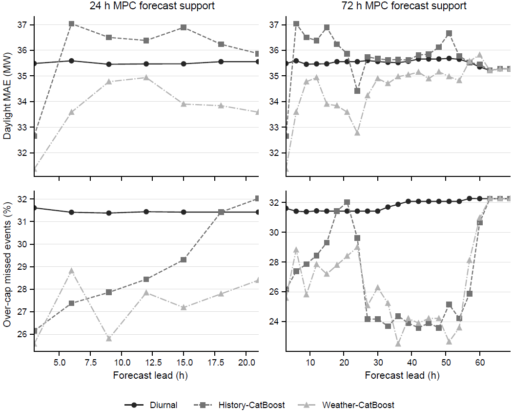
Figure S1. Leadwise forecast diagnostics
Note: Leadwise daylight MAE and over-cap missed-event rate for the three deployable forecast streams. The 24 h controller consumes leads 3–21 h, and the 72 h controller consumes leads 3–69 h.
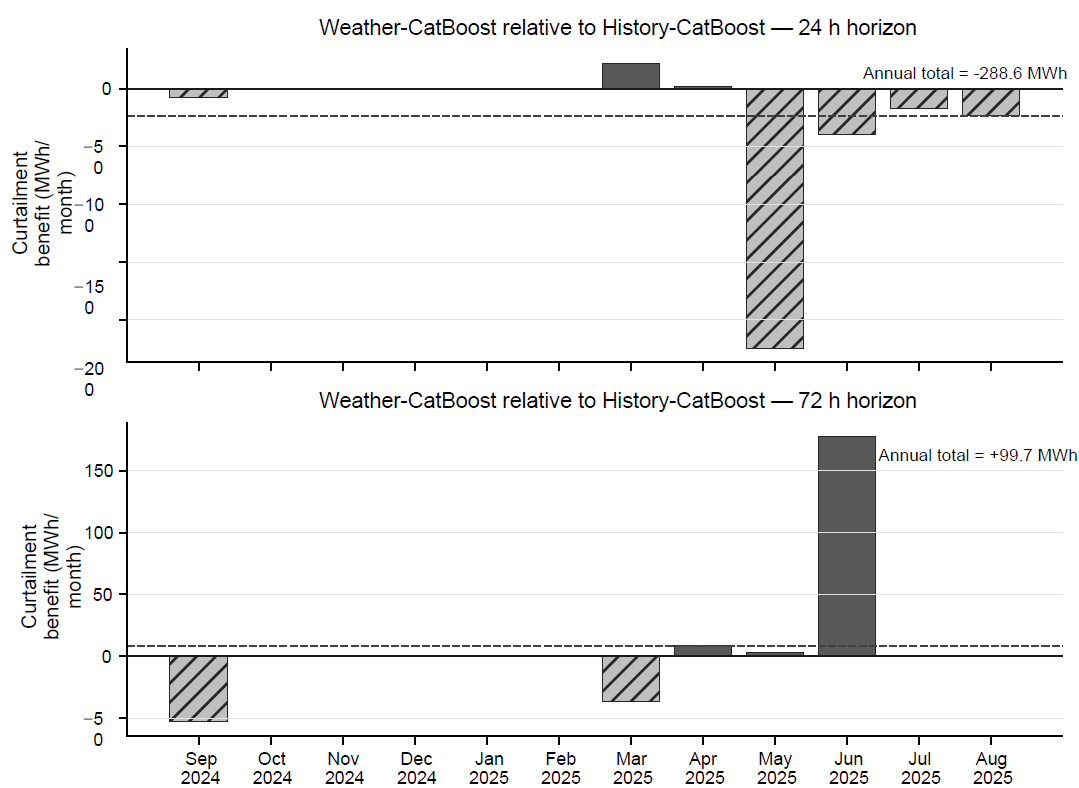
Figure S2. Monthly weather-information curtailment effect
Note: Monthly curtailment benefit of Weather-CatBoost relative to History-CatBoost. Positive values indicate lower curtailment with weather information; dashed lines show mean monthly effects.
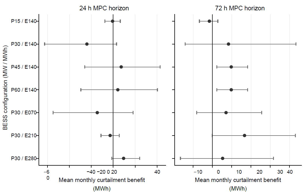
Figure S3. BESS sensitivity of weather-information value
Note: Mean monthly curtailment benefit ofWeather-CatBoost relative to History-CatBoost across independent BESS power and energy variations. Error bars are 95% circular moving-block bootstrap intervals.


 Views: 221
 Crossref: 0