Acadlore takes over the publication of JORIT from 2025 Vol. 4, No. 3. The preceding volumes were published under a CC-BY 4.0 license by the previous owner, and displayed here as agreed between Acadlore and the owner.
Testing Parallel Trends in Differences-in-Differences and Event Study Designs: A Research Approach Based on Pre-Treatment Period Significance
Abstract:
Traditional tests for parallel trends in the context of differences-in-differences are based on the observation of the mean values of the dependent variable in the treatment and control groups over time. However, given the new discussions brought by the development of the event study designs, controlling for observable factors may intervene in the fulfilment of the parallel trend assumption. This article presents a simple test based on the statistical significance of pre-treatment periods which can be extended from the classic Differences-in-Differences up to event study designs in universal absorbing treatments. The test requires at least two pre-treatment periods and can done by constructing appropriate dummy variables.
1. Introduction
Under the great development of the dynamic Differences-in-Differences (DiD) known as event studies in the recent years, new forms to test the parallel trends had emerged (See for example, Roth & Sant'Anna (2023), Rambachan & Roth (2023), and Marcus & Sant’Anna (2021) among others.). While some of them target complex relationships like the role of covariates, and the contamination of staggered adoptions (Callaway & Sant’Anna, 2021; Sun & Abraham, 2021), upon their construction they also remarked implicitly how outdated is the average trend plot by groups to inspect the parallel trends assumption. Surprisingly, a great number of economists are still not aware of how this assumption may be violated if some factors are uncontrolled under this approach, which is the case of the unconditional average value by group per year in the traditional parallel trend plot. Moreover, this classic approach can deliver wrong inferences about the existence of true parallel trends that may hold after controlling for time-varying factors (Gibson & Zimmerman, 2021) or even after the inclusion of the individual and time fixed effects.
Given the belief that some economists still have about the validity of the parallel trends with the visualization of the simple average values by groups per year (known as the traditional parallel trend plot), this article will start by denoting the visual differences that may be articulated when a set of factors are uncontrolled, and how the reaction of the trends may change once the regression framework potentially control for these factors. Furthermore, the setup of the test is presented as a middle step in the specification of the simple DiD models and the modern event study designs. Finally, based on a set of simulations, some recommendations are given in the case of individual treatment heterogeneity in the unit level which can cause a degree of heteroskedasticity and the cross-sectional size of the units that may disrupt the test.
This simple test for parallel trends requires at least two pre-treatment periods to deliver a form of statistical inference related to the differences in the trends between the treatment and control groups before the intervention. It is also necessary to work under a universal absorbing treatment, as in contrast with staggered adoptions, it can be subject to contamination (Sun & Abraham, 2021). The test is meant to be intuitive, and for such purposes is based on the creation of dummy variables that can target generic treatment effects before and after an intervention relative to a certain reference period, therefore, it is also articulated to the event study structure but in a simpler manner. The proposed test, instead of testing individual hypotheses (Roth, 2022) or the joint statistical significance of the coefficients like Callaway & Sant’Anna (2021) in the pre-treatment periods, captures the average differences in the trends through dummy variables allowing for an easier interpretation of the potential parallel trends prior an intervention. The great advantage is that it does not require complex mathematical calculations and can be carried out with simple t-tests.
This article contributes to the literature by illustrating how deprecated is the traditional parallel trend plots with unconditional means and provides a simple test for differential pre-trends in the DiD set ups for universal absorbing treatments, consistent with the structure of the event study designs. It also highlights through a set of simulations the importance of the size of cross-sectional units in both treatment and control groups to suspect potential violations of the parallel trends. The proposed test does not contribute to staggered adoption setups where some rich literature is already done, for example in Bilinski and Hatfield (2018), Freyaldenhoven et al., (2019) and Goodman-Bacon (2021).
The rest of this document goes as follows: Section 1 presents intuitively the problems of the traditional parallel trends plot based on the unconditional means by group to potentially identify parallel trends. Section 2 presents the ideal setup for the test and the core idea based on the construction of dummy variables under the regression framework while controlling for observed time-varying factors and two-way fixed effects. Section 3 presents the application of the tests in a set of simulations. Section 4 discusses some problems that can interfere with the inference of the tests along with the main conclusions.
2. The Drawback of the Traditional Parallel Trend Plot
The traditional DiD can reflect causal estimates if the parallel trend assumption is fulfilled (Lechner, 2011). Of course, this also requires other important assumptions from this specific approach, such as, no anticipation effects (Callaway & Sant’Anna, 2021), orthogonality of the treatment assignment (Khandker et al., 2009), and no dispersion/contamination of the treatment effects across groups (which is a form of sequential exogeneity). The classic way to test this parallel trend assumption (at least in the traditional DiD) is based in computing the time series averages of the outcome variable by groups over time. Resulting in the well-known “parallel trend plot” to inspect if the parallel trends hold prior the intervention. However, recent literature (Roth et al., 2023) details that these “unconditional means” calculations of the outcome, may not be ideal when confounders are present since the parallel trend may only hold true when some observable factors are controlled.
To exemplify these concepts, Figure 1 represents how much of the discrepancy can exists when the uncontrolled mean by groups of the outcome 𝑌 is plotted over time against the conditional mean of the same processes, considering as conditional factors the time and unit fixed effects through a linear trend model (Luedicke, 2022). The discrepancy is shown for both approaches in the same simulated process 𝑌~𝑁(0,1) which suffers a shock at specific time 𝑡 for some of the individuals (the treated units).

In Figure 1, panel (a) is the simple average over time for the control and treatment groups relative to the outcome 𝑌. In contrast, panel (b) is the prediction of the outcome conditional on the time and unit fixed effects under the specification of the linear trend model developed by StataCorp (2021) and explained by Luedicke (2022). The simulation has the positive shock at year 0, but the relevant part is the pre intervention which considers the set of years from -4 up to -1. It is visible that from panel (a), there is a consistent failure of the parallel trend assumption between the treatment and control groups given the visual inspection. Meanwhile on panel (b), the plot of the linear trend models, which is a model allowing to control for time and fixed specific effects, provide a better fulfillment of the assumption. As this is a simulated process, the true trends in both groups are in fact the same before the intervention.
The random process 𝑌 is in fact the same for both approaches in the pre intervention periods, but the traditional parallel trend plot in panel (a) in this example provides a wrongful inference of the behavior of the trends. The linear trend model, on the other hand, do a better job in capturing the same trends in the pre intervention periods as shown in panel (b). This example highlights how sensitive can be the unconditional means approach of the classic parallel trend plot and how important is to control for other factors to infer the parallelism of the trends in the visual inspection. Noticeable the simple and traditional trend plot using averages fails to show the parallel trends of the process 𝑌 as shown in panel (a).
In this manner, extracting trend components is an old interest of the time series econometrics branch, and the use of filters such as the Hodrick-Prescott, the Hamilton, and the Kalman filter may be used as well. However, this visual interpretation may be subjective, and therefore, some “objective” alternatives may be much better to use. These involve for example the hypothesis testing of the coefficient of the triple interaction term of the pre-intervention in the linear trend model provided by Luedicke (2022), or the use of the Callaway & Sant’Anna (2021) tests of parallel pre-trends, finally the two-way fixed effects event study plots (Marcus & Sant’Anna, 2021) can be the best alternative.
3. A Simple Test for Parallel Trends
Description and justification of the research methods used. Normally, the methods will be selected from known and proven examples. In special cases the development of a method may be a key part of the research, but then this will have been described in Introduction section and reviewed in first one.
Consider the time window of the sample which is available for both treated and control units as 𝑇,and relative to a certain event/intervention. Define the set 𝑇=[𝑎,…,−2,−1,0,1,2,…,𝑏] where 𝑎 is the first available period of the sample, and 𝑏 the last period of the window relative to the event. By defining a certain period as 𝑡∈𝑇, consider at 𝑡=0 the introduction of a universal absorbing treatment for the treated units. Now, as the set up must be compatible with the event study designs, the period 𝑡=−1 can be taken as the relative point for the estimates of the regression framework. This is where the test can be equivalent to the event study estimations, and the key is the construction of a dummy variable which captures the generic differences between the treated and control groups before and after the estimation. This approach could be thought as a variant of the linear trend model specification of Luedicke (2022) but much simpler and straightforward, and in contrast, the test is compatible with the estimates of the event study.
The test requires the definition of two dummy variables with the sole objective to capture pre and post estimation periods but without inducing perfect multicollinearity. To do so, just like in event study designs, the period 𝑡=−1 can be dropped in the construction of these dummies. Let them be defined by the next equations (1) and (2).
Under the setup of equations (1) and (2), the reference point will be placed at 𝑡=−1 as it is the excluded period. In words, (1) defines a dummy variable which has values of 1’s whenever the observation belongs to the initial period available of the sample (which is 𝑎) up to the prior year (𝑡=−2) of the relative excluded point (𝑡=−1). In the same manner, (2) is a dummy variable that contains values of 1’s whenever we are in the post intervention periods (during and after the intervention). More importantly, the dummies 𝐷(𝑡) are clearly just a function of time to identify pre and post periods relative to the mentioned reference point 𝑡=−1. With these generic dummy variables, the regression framework to test for differential parallel trend is given by:
In the previous, 𝑖 is the unit subscript and 𝑡 is the time subscript. $Y_{i t}$ is the outcome/dependent variable, $\lambda_t$ are time-specific fixed effects, $\mu_i$ are the unit-specific fixed effects, 𝛼 is the coefficient of interest for the test which captures the differences in the slopes in the pre intervention period between the treatment and control groups relative to the reference point. $D_{i t}^{P r e}$ is the dummy variable which identifies the pre intervention period according to equation (1), $T_{i t}$ is a treatment dummy variable that identifies if the unit 𝑖 has ever received the treatment or not (For completeness, the dummy identifies if unit 𝑖 is part of the treatment group, then 𝑇𝑖𝑡=1 and zero otherwise.). The coefficient 𝜏 is a measure of the generic average treatment effect on the treated after the intervention, where $D_{i t}^{ {Post }}$ is defined according to equation (2), as a dummy that identify post-treatment periods. As it is important to control for time-varying factors influencing the potential trends as stated by Roth et al. (2023), the specification also includes a set of covariates contained in 𝐗 and their respective coefficients in vector 𝜷. Finally, the residual of the model is expressed as $\varepsilon_{i t}$.
The objective in this framework is to test whether there are differential slopes in the treatment and control groups in the pre intervention period, for this purpose, the hypothesis can be stated as the simple statement $H_0: \alpha=0$ as the null hypothesis which represents the absence of significant differences in the slopes of the groups in the pre-intervention period (parallel trends hypothesis) relative to the reference period, against the alternative $H_A: \alpha \neq 0$ which implies the existence of differential pre-trends in the pre intervention period. In other words, a failure to accept the null hypothesis represents the existence of differential trends in the treatment and control groups.
Specification (3) also has important implications in the sense that neither $T_{i t}$ or $D_{i t}$ variables are placed as independent terms in the regression, the reason relies on the fact that the time and unit fixed effects will absorb them. Therefore, the interaction between the dummy periods and the treatment dummy constitutes an ideal way to capture significant differences in the pre intervention period relative to the reference point, all of them contained in average on the coefficient 𝛼. It is clear that this framework is a simplified version of the event study specifications of twoway fixed effects but a more elaborated version of the traditional DiD’s. The test, however, is sensible to some factors that must be considered: 1) Universal absorbing treatment is required. 2) At least two periods before the intervention (that is that |𝑎|≥2) are required. 3) If only two pre intervention periods exists, the number of cross-section units should be at least larger than 𝑛>30 to represent an acceptable statistical power. 4) Groupwise homoskedasticity should exists.
The previous factors are important because if there is a staggered adoption of the treatment, contamination may raise and contaminate the test, therefore, only universal absorbing treatment can deliver a useful inference of the differential pre-trends between the groups. The second is that the test works by excluding a period to be taken as reference, in this case 𝑡=−1 to avoid perfect multicollinearity, therefore it is important that the time window has at least one extra period in the pre intervention to have some plausible interpretation of 𝛼. Although the larger the pre intervention window, the better the test will capture differences over the groups. The third factor is associated with the statistical power that may exists if only one pre intervention period is available for the estimation (excluded 𝑡=−1, and available on the sample the 𝑡=−2). If only one period is taken in the estimates, then the number of cross-sectional units becomes highly important for correct inferences, and a desirable number of units independently of the classification, should be at least 30 given the nature of the t-test under the regression. Finally, if there is some existence of heteroskedasticity among the groups, the standard errors of 𝛼 may be biased, but this can be fixed by clustering the standard errors at the unit level.
4. Applications and Results
By retaking the simulation in the example of Section 2, it is possible to inspect the behavior of the test from a process which truly follows the parallel trends before the intervention. The example starts first with a large sample case and then inspects the properties by reducing both pre intervention periods and units.
Starting by a large-scale panel of 𝑛=1000 units where half of the units are part of the treatment group, this setup considers a time window of 𝑇=10 with a positive shock in the middle of window (the intervention, at 𝑡=0 of 0.5 units over the outcome 𝑌 for the treated units. Again, the outcome is generated by a normally distributed random process with 0 mean and standard deviation of 1 without covariates. Figure 1 shows the basis of this shock as a result of an intervention in the treatment group. In this sense, and to show the compatibility of the test with the standard event study designs in the form of Berge (2018), Figure 2 compiles both the event study plot and the point estimates of the general specification of (3) applied to this case.
In Figure 2, the estimation of specification (3) is successful in terms to identify the parallel trends. More specifically the redline represents the coefficient 𝛼 along with the confidence intervals at a 95% confidence level with the same color, where it touches the zero line, and represents the absence of differential pre-trends (In other words, we fail to reject the null hypothesis that α=0 with a 95% confidence level, implying the existence of parallel trends in the treatment and control group before the intervention.) for this simulation. The disaggregation of the event study plot in black color also depicts the same conclusion when the time specific effects are separated in the pre intervention period (core of the event study point estimates). Something interesting to highlight is that in the post intervention period, the null effect of the treatment dominates the generic treatment effect, even when in the event study plots the shock can be identified at year 0. The numerical result of the test is presented in the following Table 1.
Variable | Estimates | Std. Error* | t-statistic | p-value |
$\left(D_{i t}^{P r e} * T_{i t}\right)$ | α = 0.076009 | 0.073678 | 1.03164 | 0.30249 |
$\left(D_{i t}^{Post} * T_{i t}\right)$ | τ= 0.113234 | 0.069429 | 1.63093 | 0.10322 |
Table 1 presents the results of the specification in (3) where the coefficient 𝛼 captures the estimates of the potential differential pre trends in average. As noticed with the t-statistic and the p-value, we fail to reject the null hypothesis that 𝛼=0 with a 5% level of significance, implying that both groups in the pre intervention period (before 𝑡=0) behave in the same manner (thus indicating parallel trends relative to 𝑡=−1). Similar intuition it’s obtained in the post estimation period when 𝜏 is analyzed, however, the estimates do fail to identify the positive shock of the intervention. This is expected as the test is mainly based to identify differential trends given the behavior of the slopes between groups, more crucially the interest of the test is only based for the coefficient 𝛼 derived from the interaction $D_{i t}^{P r e} * T_{i t}$.
Considering the same structure with 𝑛=1000 units, but now defining the positive shock on the third period after the initial period of the time window 𝑎, this creates the extreme case where only in the estimations there is one period of information, this as a consequence of dropping 𝑡=−1 to avoid collinearity, implies that 𝑡=−2 becomes the only pre intervention period available for the estimations. The post intervention period is just increased by the periods non-used, and the results are shown in Figure 3.
By inspecting Figure 3, the red line and the respective confidence intervals are touching the zero line, indicating that the parallel trends hold before the intervention. The test in this case directly coincides with the event study point estimate and its standard error. This for the case when only one period is available in the pre intervention scenario excluding the relative period 𝑡= −1. This application of the test shows that it is a direct equivalent of the event study structure, but it is a weighted average of the magnitude of differential slopes between groups in the pre intervention period. Moreover, the post intervention generic effect is again dominated by the null difference between the groups. The respective statistics of the test are presented in Table 2 where the test over α can identify the existence of similar/parallel pre trends prior the intervention by failing to reject the null hypothesis.
Variable | Estimates | Std. Error* | T- value | P-value |
$\left(D_{i t}^{P r e} * T_{i t}\right)$ | $\alpha$ = 0.082561 | 0.088267 | 0.935351 | 0.34983 |
$\left(D_{i t}^{Post} * T_{i t}\right)$ | $\tau$ = 0.090460 | 0.067916 | 1.331936 | 0.18319 |
The results in Table 2 provide the same statistical inference about the inexistence of differential pre trends given the t-statistic and the associated p-value, where there is a failure to reject the null hypothesis of parallel pre trends at a 5% level of significance in the pre intervention period. This is in line with what was truly stated originally in the simulation. More visible, the precision of the estimates is affected by having less periods, but still the test is robust in the same statistical inference by clustering the errors at the unit level. The 𝜏 coefficient is also not statistically significant at a 5% significance level as the trends after the positive shock in 𝑡=0 remains unchanged.
The appendix presents alternative simulations to see how the response of the parallel trend test reacts in different scenarios. Section A.1 covers a special case of low sample size where 𝑛=30 with 10 treated units, and 20 control units, where the parallel trends are in fact true. The positive shock is also allocated in the middle of the time window 𝑇, the results evidence that the test also performs quite well when the sample size is not large. The results in Figure 4 and Table 3 over the t-statistic of the 𝛼 coefficient fail to reject the null hypothesis of parallel pre trends with a 5% level of significance.
Other special case is a false positive scenario (Section A.2) under a large-scale sample, where the data generating process in fact contains differential pre-trends. To identify if the test over 𝛼 is able to discover differential pre-trends, this simulation is carried with a negative pre-trend from the treatment group in periods -4, and -3, but a normalization in periods -2 and -1 as a reflection of anticipation effects. Therefore, the differential pre-trends are only present in periods -4 and -3. The setup contains a large-scale panel just like the first simulation with a positive 0.5 unit shock over the treatment group in the middle of the time window 𝑇, and the result shown in Figure 5 and Table 4 provide evidence that the test over 𝛼 is able to identify the differential pre-trends, even when the normalization (as a form of anticipation effects) is present in periods -2 and -1. Specifically in Table 4, there is a rejection of the null hypothesis of the 𝛼 coefficient of parallel trends in the pre intervention period statistically significant with a 1% level of significance.
Finally, a small sample false positive scenario is simulated (Section A.3), similar to the previous one but instead of a large-scale number of units, this one in contrasts contains only 10 treated units and 20 control units and the results are in Figure 6 and Table 5. The test over 𝛼 fails to reject the null hypothesis of parallel trends at a 5% level of significance, but over a 1% significance levels, depicts the existence of differential pre-trends. This case exemplifies the sensibility of the test when the number of cross-sectional units is relatively small (𝑛=30), which is a situation that can be associated with the problems described by Bilinski and Hatfield (2018). Nevertheless, the test with a stricter level of significance is able to detect the differential pre-trends. In this sense, if the statistical significance of the test displays the rejection over a 99% confidence level, it may be worth to create the event study specification in terms of Berge (2018) to confirm the results in the existence of individual time heterogeneity.
5. Limitations and Conclusions
The parallel trend test presented in this article can be thought as a mirror of the average generic effects of the event study estimates. The test is generally able to identify the existence of parallel trends by failing to reject the null hypothesis of parallel pre trends in the slopes of the treatment and control groups under a universal absorbing treatment. The test, however, display a sensitivity due to the number of the cross-sectional units as it depends on the t-statistic for the inference, and thus it is recommended to be applied when these cross-sections are not small (at least larger than 30 units across treatment and control groups). The false positive tests with different sample sizes confirm this weakness. And thus, when the rejection of the null occurs with a stricter significance level (e.g., 1%), it is recommended then to inspect the period specific point estimates in the event study form of Berge (2018), as the proposed test is compatible with these point estimates.
More importantly, this article also exemplified the weakness of the traditional parallel trend plots in the light of the event study designs, where the proposed test of parallel trends is simple to carry out and only requires the construction of dummy variables to identify the pre and post intervention periods considering the exclusion of a relative point in time (in this case t =-1) just like in the event study designs. The test requires at least two periods of information before the event, and the results are robust in the presence of heteroskedasticity by clustering the standard errors at the unit level. This test contributes to the existing literature in the discussion of parallel trends by providing an alternative to other tests like the ones presented in the linear trend models or the joint hypothesis testing of event study coefficients, as the proposed test can capture the dominant weighted behaviour of the trends between the groups in universal absorbing treatments.
The author performed all tasks involved in manuscript preparation, research, and writing.
Special thanks to Dr. Uwe Sunde, Dr. Ilka Gerhardts, my colleagues Till Wiedermann and Michael Reindl of the Ludwig-Maximilians-Universität for their comments and feedback regarding the topic of event study designs during my thesis. This research was not funded or financially related. I declare there is no financial or other substantive conflict of interest that could be seen to influence your results or interpretations.
The author declares that the research was conducted in the absence of any commercial or financial relationships that could be construed as a potential conflict of interest.
A1. Test with small number of cross-section units
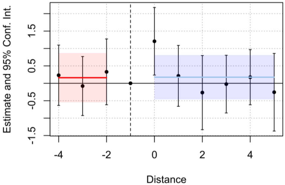
Figure 4. Event study plot with generic treatment effects (n=30)
Source: Own elaboration.
Table 3. Results of the test (n = 30, 10 treated units, 20 control units)
Variable | Estimates | Std. Error* | T- value | P-value |
$\left(D_{i t}^{P r e} * T_{i t}\right)$ | 𝛼 = 0.160616 | 0.346483 | 0.463562 | 0.64642 |
$\left(D_{i t}^{Post} * T_{i t}\right)$ | 𝜏= 0.175124 | 0.311405 | 0.562367 | 0.57819 |
Note: * Robust standard errors clustered at the unit level.
Source: Own elaboration.
A2. Test with a false positive and large sample
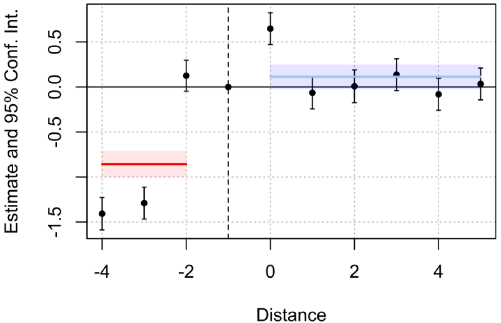
Figure 5. False positive, event study plot with generic treatment effects (n=1000)
Source: Own elaboration.
Table 4. Results of the test of false positive (n=1000, 500 treated units, 500 control units)
Variable | Estimates | Std. Error+ | T- value | P-value |
$\left(D_{i t}^{P r e} * T_{i t}\right)$ | 𝛼 = -0.857 | 0.073678 | -11.63605 | 2.2e-16*** |
$\left(D_{i t}^{Post} * T_{i t}\right)$ | 𝜏= 0.113234 | 0.069429 | 1.63093 | 0.10322 |
Note: *** Significant under a 99% level of confidence. + Robust standard errors clustered at the unit level.
Source: Own elaboration.
A3. Test with false positive and small sample
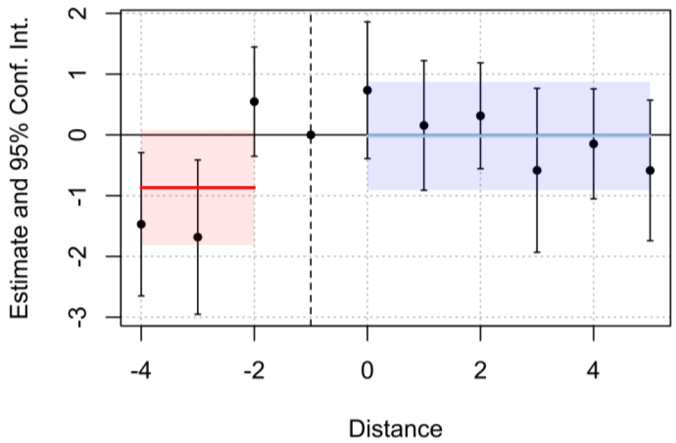
Figure 6. False positive, event study plot with generic treatment effects (n=30, 10 treated, 20 control)
Source: Own elaboration.
Table 5. Results of the test of false positive (n=30, 10 treated units, 20 control units)
Variable | Estimates | Std. Error+ | T- value | P-value |
$\left(D_{i t}^{P r e} * T_{i t}\right)$ | 𝛼 = -0.868525 | 0.462300 | -1.878703 | 0.070371* |
$\left(D_{i t}^{Post} * T_{i t}\right)$ | 𝜏= 0.113234 | 0.069429 | 1.63093 | 0.10322 |
Note: + Standard errors clustered at the unit level. * Significant under a 90% level of confidence.
Source: Own elaboration.