Data-Driven Demand Forecasting for Retail Decision-Making: A Hybrid Machine Learning and Time Series Approach to Inventory Optimization

Effective inventory management is fundamental to modern retail operations, ensuring that products are available when and where customers need them while balancing stock levels with operational costs [1-2]. In large-scale retail networks such as Walmart, this balance is particularly difficult to achieve due to complex demand patterns, seasonality, promotions, and regional variability [3]. Inaccurate demand forecasting often leads to stockouts and overstocking, resulting in financial losses, inefficient resource utilization, and diminished customer satisfaction. Consequently, improving forecasting accuracy is not only a predictive task but also a critical enabler of effective data-driven decision-making across retail operations.

Recent advances in machine learning (ML) have shown strong potential in enhancing forecasting performance by capturing nonlinear relationships, temporal dynamics, and the influence of external variables [4-6]. Building on these developments, this study aims to advance demand forecasting by systematically integrating a wide range of approaches, including time series models, regression techniques, deep learning (DL) architectures, and novel hybrid and hierarchical hybrid frameworks. A key contribution of this research is the application of automated machine learning (AutoML) to evaluate and rank multiple forecasting models, including 18 time series models and 17 regression models, using standardized performance metrics. In addition, deep learning models are optimized through a grid search strategy across five architectures to ensure robust model configuration.

Beyond methodological advancement, this study emphasizes the role of forecasting as a decision-support tool. Unlike prior research that primarily focuses on predictive accuracy, this work explicitly links forecasting outputs to operational, tactical, and strategic decision-making processes. At the operational level, improved forecasts support replenishment planning, safety stock optimization, and inventory control. At the tactical level, they enable more effective distribution planning, workforce scheduling, and demand-driven logistics. At the strategic level, accurate demand insights contribute to supply chain design, capacity planning, and long-term resource allocation. This integrated perspective positions forecasting as a central component of data-driven retail decision systems.

Furthermore, the study introduces a hierarchical hybrid framework that combines deep learning forecasts with residual modeling and store-level aggregation to enhance prediction accuracy across multiple levels of analysis. Comprehensive data preprocessing and imputation techniques are employed to improve data quality and model robustness. By consolidating diverse forecasting approaches within a unified framework, this research enables direct comparison of methods and provides deeper insights into their practical applicability.

The primary objectives of this study are to:

$\bullet$ Enhance forecasting accuracy by capturing temporal dynamics and external demand drivers;

$\bullet$ Evaluate and compare multiple ML techniques using Walmart’s historical sales data to support informed inventory decisions;

$\bullet$ Develop hybrid and hierarchical hybrid models that facilitate data-driven decision-making at both aggregate and store levels.

The remainder of this paper is organized as follows: Section 2 reviews relevant literature; Section 3 details the methodology, including data preparation, experimental design, and evaluation metrics; Section 4 presents and analyzes the results and discusses the practical implications for organizational decision-making; and Section 5 concludes with a discussion of key findings and implications for retail demand forecasting.

Several research studies have explored the use of ML models on Walmart's historical weekly sales dataset [7] to improve demand forecasting accuracy. Yang [8] investigated the performance of three popular models: Ordinary Least Squares (OLS) regression, Random Forest (RF), and Extreme Gradient Boosting (XGBoost). He found that XGBoost outperformed the other models in predictive accuracy due to its ability to handle skewed data and non-linear interactions. In a similar study, Yao [9] compared Decision Tree, RF, and K-Neighbors Regressor models. His research concluded that RF delivered the most accurate results, highlighting its robustness in capturing complex patterns in the data, particularly non-linear relationships. Yi [10] extended this exploration by using Linear Regression, RF, and XGBoost further emphasizing the importance of feature engineering and hyperparameter tuning. His findings confirmed that XGBoost provided the best sales predictions. Lastly, Akande et al. [11] focused solely on the XGBoost algorithm and showed that it offered superior predictive accuracy when optimized with comprehensive data preprocessing and feature selection. Table 1 summarizes the findings and limitation of this four studies.

Beyond the exploration of Walmart's dataset, other studies have applied time series and DL models to improve demand forecasting and inventory management across various sectors. Praveen et al. [12] proposed an XGBoost regression model for inventory demand forecasting in small and medium-sized businesses, focusing on optimizing inventory levels by accurately predicting short-term demand. Similarly, Purnamasari et al. [13] utilized models such as Seasonal Autoregressive Integrated Moving Average (SARIMA), Seasonal Autoregressive Integrated Moving Average with External Factors (SARIMAX), Long Short-Term Memory (LSTM), XGBoost, and Gaussain Process Regression for demand forecasting in small and medium enterprises, with their findings highlighting XGBoost’s superior accuraccy, making it highly effective for inventory management. In the field of supply chain management, El Filali et al. [14] implemented an optimized LSTM network, demonstrating that fine-tuning the LSTM architecture using a grid search algorithm significantly improves demand forecasting accuracy and inventory efficiency. Their proposed model outperformed statistical and ML models such as Exponential Smoothing (ETS) and Autoregressive Integrated Moving Average (ARIMA). Additionally, another study conducted by Bashaer and Belal explored demand forecasting for medicine, comparing various DL techniques including Recurrent Neural Network (RNN), LSTM, Bidirectional LSTM, and Gated Recurrent Unit (GRU), with their RNN model achieving the best accuracy for managing pharmaceutical inventory [15]. These studies collectively underscore the adaptability and strength of sequential models for enhancing demand forecasting across multiple industries. However, a limitation of these models is their difficulty in effectively capturing external regression factors like promotions, economic indicators, and weather conditions, which can significantly influence demand [16].

In addition to the extensive application of ML and DL models for demand forecasting hybrid approaches have also shown significant promise. Punia et al. [17] introduced a hybrid methodology that integrates LSTM networks with RF to enhance demand forecasting in multi-channel retail environments. By using LSTM networks to capture temporal dependencies and RF to model residuals accounting for non-temporal factors such as promotions and holidays, the study demonstrated superior forecasting accuracy compared to traditional models like ARIMAX or standalone LSTM and RF models. In a related study by Taghiyeh et al. [18] proposed a child-level forecasts specifically tailored for hiearchical supply chain management. Their methodology uses ML models such as Multi-Layer Perceptron, RF, GBM, and XGBoost to forecast demand at various hierarchical levels. The multi-phase hierarchical approach refines and aggregates forecasts across different levels of the supply chain, achieving a 82-90\% reduction in forecasting errors compared to traditional forecasting methods. The study highlights the efficacy of hierarchical methods in improving demand forecasting accuracy and efficiency across complex supply chains.

Building on the strengths of both hybrid and hierarchical methodologies, this study introduces a hierarchical hybrid modeling framework that integrates DL techniques with regression models while also forecasting at a granualar levels. This combined strategy captures both temporal dependencies and external influencing factors, leading to enhanced forecasting accuracy and improved operational efficiency across Walmart’s store network. Table 2 offers a comparative summary of the modeling strategies explored highlighting their implementation, previously identified limitations, and the distinct innovations contributed by this work.

The methodology for this study is inspired by the CRISP-DM (Cross-Industry Standard Process for Data Mining) framework [19], which provides a structured approach to data mining and ML projects. Although not every step of the CRISP-DM process is followed in detail, its principles guide the overall workflow. The project begins with a business understanding phase followed by a data description phase, which includes data understanding, preprocessing, exploratory data analysis (EDA), and data preparation. The core of the methodology is the modeling phase, where five distinct experiments: time series analysis, regression models, DL techniques, hybrid approach, and hierarchical hybrid approach, are conducted to explore different facets of the forecasting problem. The performance of these models is then assessed during the evaluation phase to identify the most accurate and robust model. Finally, in the future forecast phase, the trained models are used to predict sales for the next year, providing actionable insights for inventory management and strategic planning. This workflow ensures a thorough and systematic approach to demand forecasting, which is detailed in the subsequent sections.

This study utilizes Walmart’s historical weekly sales data, which covers 45 stores in US over a period of 182 weeks. The dataset consists of detailed store information, sales figures per departement, and external factors such as weather conditions and economic indicators. This section provides a comprehensive overview of the key data sources, which are organized into four main files: Stores, Features, Train, and Test.

The Stores dataset offers a high-level overview of 45 Walmart stores, detailing their ID, type, and size across 45 rows and 3 columns. Each store is identified by a unique ID (1–45) and categorized by type (A, B, or C), with type A stores generally larger and type C stores smaller, as indicated by a strong negative correlation between Type and Size. The dataset is complete, with no missing or duplicate values.

The Features dataset provides weekly data for each Walmart store over a span of 182 weeks from February 2010 to July 2013, with 8,190 rows and 12 columns that capture both store specific and external factors. Key variables include Temperature, Fuel\_Price, MarkDown1 to MarkDown5, CPI (Consumer Price Index), Unemployment, and IsHoliday. These features help explain fluctuations in consumer behavior and sales performance. The five types of markdowns represent Walmart's promotional strategies, such as price cuts on clearance items, discounts, buy-one-get-one-free offers, rollbacks, and 10\% off for new members. The CPI measures the overall cost of goods and services, while the unemployment rate is the percentage of the labor force that is actively seeking work but currently unemployed, both of which impact consumer spending behavior. However, the dataset contains missing values in the CPI, Unemployment, and MarkDowns columns, which could potentially distort the model's ability to predict sales accurately if not handled appropriately.

The Train dataset includes historical weekly sales for various departments across 45 Walmart stores, featuring 81 unique departments identified by IDs ranging from 1 to 99, though some department IDs are missing, indicating gaps in the data for certain departments. It consists of 421,570 rows covering a period of 143 weeks, from February 2010 to October 2012. The sales data shows a wide range of variability, from negative amounts to over half a million dollars, highlighting substantial differences in performance across departments. The distribution of weekly sales is heavily right-skewed, as shown in Figure 1, indicating that the majority of sales values are concentrated at the lower end of the sales range, closer to zero. Most weekly sales fall below 100,000, with the highest frequency occurring near 0, reflecting that many departments have moderate weekly sales. However, a small number of instances show much higher sales, ranging from 100,000 to over 600,000 though these are far less frequent, indicating that while most weeks experience moderate sales, certain periods see significant spikes.

The number of departments varies by store, with some managing more than others, and inconsistencies exist in data entries per store and department, indicating areas needing further preprocessing. These insights into the Train dataset’s structure emphasize its complexity, underscoring the importance of thorough data preparation for building accurate and reliable demand forecasting models.

The Test dataset mirrors the Train dataset but excludes the Weekly Sales column. It spans 39 weeks, from November 2012 to July 2013, with each row representing a department in one of the 45 Walmart stores. This dataset is used to predict future sales.

Initial analysis of Walmart’s sales data reveals several issues affecting forecast reliability, including missing values, inconsistencies, and anomalies such as negative entries. This section outlines the preprocessing steps used to clean the data and engineer relevant features for improved model performance.

(1) Handling missing values

The MarkDown1 to MarkDown5 columns contain missing values, from February 2010 to November 2011. To address this, a mapping approach was used to impute missing values based on markdown data from 2012, assuming similar sales patterns across these periods [20]. This process involved four key steps: first, splitting data into valid entries from 2012 and missing data from 2010–2011; second, mapping missing dates to equivalent weeks in 2012; third, assigning markdown values from 2012 to these gaps; and finally, filling any remaining gaps with zeros, under the assumption that no markdowns occurred during unrecorded periods.

Both the CPI and Unemployment columns have missing values for the last 13 weeks of the dataset in 2013. To resolve this, an ARIMA time series model is applied to the available CPI and unemployment data for each store. ARIMA models are effective for forecasting time series data by capturing patterns of autocorrelation and trends, combining autoregression, differencing to make the data stationary, and moving averages to account for past forecast errors [21]. Using this approach, the missing CPI and unemployment values are predicted and integrated into the dataset, ensuring continuous and complete records across all weeks and stores.

(2) Data cleaning

The first step involves the removal of negative sales values. The train dataset initially contains 1,285 rows with negative values, which are not realistic for sales data. These entries are removed, reducing the dataset to 420,285 rows, ensuring that all sales figures are valid and positive. Next, stores with insufficient or inconsistent data patterns are dropped. After evaluating the weekly sales and data entries per store, nine stores—30, 33, 36, 37, 38, 39, 42, 43, and 44—are removed from both train and test datasets. Further cleaning involves dropping departments with incomplete data. Departments with fewer than 143 unique weeks are considered incomplete. As a result, departments such as 6, 16, 18, 19, 32, 35, 36, 37, 39, 41, 43, 45, 47, 48, 49, 50, 51, 54, 56, 58, 59, 60, 65, 77, 78, 80, 83, 93, 94, 96, 97, 98, and 99 are removed. Finally, the IsHoliday column is dropped as it duplicates holiday information already available in the features dataset. After these cleaning steps, the final train dataset contains 247,104 rows, covering 48 departments across 36 stores. Both datasets, train and test, are now consistent, complete, and ready for further analysis and modeling.

(3) Feature engineering

Feature engineering consist of creating new variables that can improve the accuracy of the sales forecasting models. By deriving meaningful features from the available data, we ensure that the models can capture complex patterns and relationships that may influence sales.

$\bullet$ Total Markdown: The original dataset contains five separate markdown columns representing different promotional activities. To simplify the modeling process and provide a single metric that encapsulates all promotional effects, a new feature called Total Markdown is created. This feature consolidates the values from the five markdown columns into one, representing the overall promotional activity for each week.

$\bullet$ Holiday Type: The original IsHoliday feature indicates whether a given week is a holiday or not but lacks further detail. To refine this, holidays are categorized into specific events, such as the Super Bowl, Thanksgiving, Labour Day, and Christmas. A new feature, Holiday Type, is introduced to represent these distinct events numerically. This transformation provides the model with more granular information on the type of holiday, which could have varying effects on sales patterns. For instance, sales dynamics during the Super Bowl may differ significantly from those during Christmas, and this feature helps capture those variations.

$\bullet$ Season: To account for the seasonal variations in sales, a new Season feature is derived from the month of the year. This column categorizes the time of year into four seasons: Winter, Spring, Summer, and Fall. Given that consumer behavior varies greatly across seasons, with sales peaking during the holiday season or summer promotions, this feature adds another layer of predictive power to the model by helping it better understand seasonal trends in sales.

The EDA provides valuable insights into the impact of various features on Walmart’s weekly sales across different levels [22]. By merging datasets, the analysis reveals trends, seasonal patterns, and feature influences, helping to pinpoint key drivers of sales.

(1) Sales trends over time

Analysis of total weekly sales ( Figure 2a) reveals a strong seasonal pattern, with noticeable peaks at the end of the year driven by holiday shopping. During these periods, sales reach their highest volumes, while they stabilize between peaks, maintaining a consistent range between \$35 million and \$40 million weekly. Sales by store type ( Figure 2b) show that Type A stores consistently outperform Type B, likely due to their larger size and broader product range. At the store level ( Figure 2c), seasonal trends are common, though baseline sales vary by location, likely influenced by factors such as demographics, store size, and customer behavior.

(2) Features influence on sales

The analysis of the features influencing weekly sales is presented in Figure 3 and Figure 4. Starting with the Season, the average weekly sales across different seasons ( Figure 3a) show that winter has the highest sales, likely driven by holiday shopping, while spring experiences a drop in spending. Summer sees a slight recovery, and fall benefits from early holiday preparations. The seasons are encoded as 1 for winter, 2 for spring, 3 for summer, and 4 for fall. Next, the average weekly sales by temperature category ( Figure 3b) shows the sales performance across different temperature levels, where 1 represents low, 2 represents medium, and 3 represents high temperatures. The chart indicates that medium temperatures are linked to the highest sales, likely because moderate weather encourages more consumer activity. In contrast, both low and high temperatures see reduced sales, with cold weather having the most significant negative impact on shopping activity. The average weekly sales across holiday types ( Figure 3c) show how different holidays impact sales, where 1 represents the Super Bowl, 2 represents Labour Day, 3 represents Thanksgiving, and 4 represents Christmas. The chart indicates that Thanksgiving is the most commercially impactful holiday, generating the highest weekly sales, likely due to Black Friday occurring in the same week. This is followed by the Super Bowl, with Labour Day coming in third. Surprisingly, Christmas records the lowest weekly sales, possibly because peak sales occur in the weeks leading up to the holiday rather than during the holiday week itself.

The analysis of economic indicators (Figure 4) reveals weak linear relationships between weekly sales and variables like unemployment, fuel prices, and CPI, with sales widely distributed across different levels of these indicators. This suggests that external economic factors have limited direct influence on sales, while internal factors play a more substantial role in driving sales performance.

To effectively prepare the data for sales forecasting, two levels of aggregation are performed. The first level of aggregation focuses on calculating total weekly sales across all Walmart stores. This involves summing the sales data from each week across all stores and departments, resulting in a simplified dataset with 143 rows, one for each week. The total weekly sales range between approximately 30 million (3.09e+07) and 65 million (6.49e+07). Key features are processed accordingly: temperature, fuel prices, CPI, and unemployment are averaged across all stores to capture general economic and environmental conditions. Season and HolidayType are retained as the first available value for each week, assuming consistency for these categorical features, and Total Markdown is summed to reflect the overall promotional activity during each week. This aggregated dataset provides a high-level view of sales trends, offering a comprehensive summary of how various factors influence Walmart’s total sales across the country.

The second level of aggregation preserves store-level granularity by calculating total weekly sales for each store, resulting in a dataset with 5,434 rows. This approach allows for a detailed analysis of sales trends at the individual store level. Feature processing follows the same strategy as the first aggregation, enabling localized analysis while maintaining consistency in data structure.

The modeling phase of this study comprised five experiments exploring different approaches to sales forecasting: time series models, regression models, deep learning, a hybrid approach, and a hierarchical hybrid approach. The objective is to identify the most effective strategy for forecasting weekly sales across Walmart stores, both in aggregate and individual store level.

Automated ML (AutoML) is a rapidly evolving field that aims to simplify the process of developing ML models by automating the selection, training, and tuning of algorithms [23]. AutoML tools have made it significantly easier for both experts and non-experts to develop high-performing models without requiring deep technical knowledge allowing them to efficiently build and compare multiple models without manually configuring each of them [24]. This automation streamlines the modeling process, enabling quicker iterations and often leading to the discovery of models that perform exceptionally well with minimal human intervention. The PyCaret library in Python automates the training and comparison of time series and regression models, ranking them by Mean Absolute Error (MAE). The dataset, comprising aggregated weekly sales data from Walmart stores, is scaled using min-max scaling for both target and exogenous variables, ensuring all features fall within a 0–1 range to improve model convergence [25]. The date is set as the index to maintain temporal integrity, and the data is split into a training set (first 135 weeks) and a test set (last 8 weeks).

(1) Time series modeling using AutoML

In the first experiment, time series models are trained to forecast walmart total weekly sales. The models are evaluated using an expanding window cross-validation strategy with three folds. In this strategy, the training set starts small and grows with each step, while the validation set always stays in the future. This approach helps ensure that the model is only trained on past data and tested on future data, which prevents information from leaking between training and testing. PyCaret provides access to 18 time series models, including Extra Trees, Random Forest, AdaBoost, Gradient Boosting, Auto ARIMA, and Ridge Regression, among others. Figure 5 illustrates the automated process for setting up and evaluating time series models.

(2) Regression modeling with AutoML

In the second experiment, PyCaret is used to train and compare regression models for predicting Walmart total weekly sales. To ensure temporal consistency, a time series split strategy with three folds is applied for cross-validation. Unlike random cross-validation, this method maintains the sequence of the data, training on past observations and testing on future ones. This approach prevents data leakage and better simulates real-world forecasting by ensuring the model is evaluated on unseen future data. Using three folds ensures a robust evaluation, with the training set growing progressively with each fold. 17 different regression models, including Random Forest Regressor, Gradient Boosting Regressor, Extra Trees Regressor, and AdaBoost Regressor, are automatically trained and ranked. Figure 6 outlines the key steps involved in the automated setup and evaluation of regression models using PyCaret.

The use of AutoML significantly reduces the time required to evaluate multiple models, providing optimal results for both time series and regression based approaches without the need for manual hyperparameter tuning. The MAE is used as the primary evaluation metric to ensure consistency in performance comparison across different modeling approaches.

In this third experiment, multilayer RNN, single-layer LSTM, multilayer LSTM, bidirectional LSTM, and GRU models are implemented and compared to predict total weekly sales. RNNs are neural networks designed specifically for sequential data, making them well-suited for time series forecasting [26]. They maintain a memory of previous inputs, helping to model temporal dependencies. However, standard RNNs often struggle with long-term dependencies due to the vanishing gradient problem, which causes the gradients of the loss function to become extremely large during training in certain cases, leading to inefficiencies in both the training process and the resulting network [27]. To address this, LSTM networks were developed with mechanisms called gates that regulate the flow of information, allowing them to retain information over longer periods [28]. Bidirectional LSTMs extend this capability by processing data in both forward and backward directions, capturing dependencies from both the past and future relative to a specific time step [29]. GRUs, a simplified version of LSTMs, combine the forget and input gates into a single gate, making them faster to train while still effectively handling long-term dependencies [30]. The same process is used to build and evaluate the different models, with the primary difference being the layer architecture of each model. This process is illustrated in Figure 7.

Each model is implemented using TensorFlow. The process begins with data preparation, which involves splitting the data into training and test sets, where the first 135 weeks are used for training and the last 8 weeks for testing. The data is then further divided into features, which are the input variables, and the target, which is the output variable. Next, data normalization is applied using the MinMaxScaler to scale the features into the range of 0 to 1. Data normalization is crucial for deep learning model training as it ensures that all features have the same scale, preventing features with larger ranges from dominating the learning process and speeding up the convergence of the optimizer [31]. Following this, sequences of four time steps are created, which is essential for time series modeling as it allows the model to capture sequential dependencies, meaning the sales of the past four weeks are used to predict the sales for the next week. After data preparation, the models are built layer by layer. Each model employs dropout regularization to prevent overfitting, which randomly deactivates a fraction of neurons during training to make the network more robust. The Adam optimizer, an optimization algorithm that dynamically adjusts the learning rate [32], is used for training due to its efficiency with complex networks. The MAE is selected as the loss function, chosen for its simplicity and its ability to minimize the impact of outliers [33], ensuring the model focuses on reducing the overall prediction error. Initially, the number of units (neurons) in each layer is set to 50, and the dropout rate to 0.2. To fine-tune the hyperparameters for each model, the Grid Search algorithm is implemented. Grid search is an exhaustive search method that evaluates every possible combination of a set of hyperparameters to identify the best performing configuration [34]. It systematically tests different values of the hyperparameters, training the model for each combination, and then selects the one that results in the best performance based on a specific evaluation metric, which in this case is the MAE. The hyperparameters tested during the grid search include the number of units, which refers to the neurons in the hidden layers, dropout rates, which prevent overfitting by randomly deactivating certain neurons during training, batch sizes, which represent the number of training samples processed before updating the model’s parameters, and the number of epochs, which determine how many times the model sees the entire dataset during training. These parameters are detailed in Table 3.

By evaluating all combinations of these hyperparameters, grid search allows for a comprehensive exploration of the model’s possible configurations, ensuring that the final model is well-tuned for the specific data and problem at hand. This process is computationally intensive but crucial for achieving optimal performance. Finally, the models are used to forecast future sales based on the learned patterns.

The hybrid modeling approach integrates the strengths of DL based time series models and RF model to improve the accuracy of sales forecasting. The workflow followed to build the hybrid model is illustrated in Figure 8.

After identifying the best-performing sequential model, the focus shifts to residual modeling. Residuals calculated as the difference between actual sales and predicted sales from the time series model are then modeled using a RF model (n\_estimators = 100, random\_state = 42). In this step, additional external features, such as temperature, season, CPI, unemployment rates, fuel prices, markdowns, and holiday type, are incorporated. These external factors help capture the effects that may not have been fully accounted for by the time series models. The final sales prediction is obtained by summing the outputs of the best time series model and the regression model. This hybrid approach combines the strengths of both sequential and regression models to provide a more accurate and comprehensive prediction.

This approach begins by leveraging DL models, such as LSTM, Bidirectional LSTM, and GRU networks, to predict total weekly sales. The best-performing model is selected based on its MAE, using a fixed set of hyperparameters presented in Table 4. Adam is used as the optimizer, and MAE as the loss function. The last 8 weeks of data are designated as the test set to validate the model's performance, using only the weekly sales as feature at this stage.

The final experiment builds upon the previous hybrid model for aggregate weekly sales forecasting by refining it to predict weekly sales at the individual Walmart store level. This hierarchical hybrid modeling approach is designed to capture both the temporal dependencies present in time series data and the influence of external factors on sales at the store level. By modeling each store independently, the method accounts for local variations and store-specific drivers that may not be captured in an aggregate model. To assess the overall effectiveness of this hierarchical hybrid approach, the predicted sales for all stores are aggregated, allowing for a direct comparison with the total sales forecasts generated by earlier models, as illustrated in Figure 9.

To assess the performance and accuracy of the various forecasting models developed in this study, three evaluation metrics are employed: MAE, Root Mean Squared Error (RMSE), and the R-squared (R$^2$) coefficient [35]. MAE, expressed in Eq. (1), measures the average magnitude of errors in a set of predictions, without considering their direction.

where, $y_i$ represents the actual values, $\hat{y}_i$ represents the predicted values, and $n$ is the number of observations. MAE is particularly useful because it provides a clear interpretation of the average error in the same units as the target variable, making it easy to understand and communicate.

RMSE (Eq. (2)) quantifies the difference between predicted and actual values, giving more weight to larger errors.

RMSE is useful for understanding how well the model performs with respect to larger errors, which can be critical in applications where large deviations are particularly undesirable.

The R-squared coefficient Eq. (3) measures the proportion of the variance in the dependent variable that is predictable from the independent variables.

where, $\bar{y}_i$ is the mean of the actual values. R$^2$ provides an indication of how well the model fits the data, with a value of 1 indicating a perfect fit. It is particularly helpful in comparing the explanatory power of different models.

This section presents and analyzes the results of the experiments. The following subsections detail the performance of each model, accompanied by a discussion on the implications of these findings for sales forecasting.

The first experiment involves the application of 18 different time series models using the PyCaret AutoML library. Table 5 summarizes the performance metrics of the top 2 performing models, the Extra Trees Regressor and the AdaBoost Regressor.

The Extra Trees Regressor, an ensemble learning method that builds multiple decision trees and merges their results to improve predictive accuracy and control overfitting, achieves a lower MAE, indicating slightly better performance in minimizing absolute prediction errors compared to AdaBoost. On the other hand, the AdaBoost Regressor, which combines multiple weak learners into a strong one by focusing on correcting the errors of prior models, demonstrates a higher R² value, suggesting it explains more variance in the sales data. To further evaluate the models' predictive power, the forecast is extended to the following year's sales, comparing the models' out-of-sample predictions with actual sales data. Figure 10 illustrates the forecasting performance of the Extra Trees Regressor and AdaBoost Regressor over the next year.

As depicted in Figure 10, both models capture the general sales trends, including the seasonal peaks associated with major holidays. However, the Extra Trees Regressor provides more stable predictions, aligning closely with the observed sales patterns.

In the second experiment, 17 regression models are applied using the PyCaret AutoML library. Table 6 presents a summary of the performance metrics for the top two models: the Random Forest Regressor and the Gradient Boosting Regressor.

The Random Forest Regressor, which builds an ensemble of decision trees and averages their predictions, exhibits a relatively high MAE and RMSE, alongside a strongly negative R² value. These results indicate that the model struggles significantly to capture the underlying sales patterns, likely due to the complexity and variability in the data. Similarly, the Gradient Boosting Regressor, which builds trees sequentially to correct errors from previous iterations, also yields poor performance, with even higher MAE and RMSE values and a negative R² score. Despite their poor performance, these two models rank as the top two regression models based on their MAE values. However, the negative R$^2$ values for both models suggest that they perform worse than a simple mean-based prediction, indicating that these regression models fail to capture the temporal dependencies and variability in the sales data effectively. The future forecasting plots presented in Figure 11 illustrate the predicted weekly sales using the two models for the year following the training period.

Both models exhibit similar overall trends in their forecasts, but neither successfully captures the spikes in sales, particularly around peak periods. The Random Forest Regressor demonstrates some alignment with the actual sales trend, though it smooths out key fluctuations, failing to reflect the sharp sales peaks that occur during specific seasons or events. The Gradient Boosting Regressor, while generally aligned with the trend, also struggles to mimic these critical spikes. This limitation is likely due to the sequential nature of Gradient Boosting, which focuses on correcting prior errors but may not adequately adjust for sharp, irregular variations in the data. These results suggest that both models are inadequate for capturing the full complexity of the sales data, particularly the significant fluctuations that play a crucial role in retail forecasting.

In the third experiment, Multilayer RNN, Single Layer LSTM, Multilayer LSTM, Bidirectional LSTM, and GRU models are applied to forecast total weekly sales. A grid search algorithm is utilized to fine tune the hyperparameters, selecting the best configuration for each model. Table 7 summarizes the optimal hyperparameters identified through the grid search for each of the DL models used in the study.

Table 8 presents the performance metrics for each model on both the original and normalized data.

The Multilayer RNN shows the weakest performance, with the highest MAE, RMSE, and a negative R$^2$, indicating its difficulty in capturing the complexity of the sales data. The Multilayer LSTM performs better, with lower MAE and RMSE, demonstrating its ability to capture long-term dependencies. The Single Layer LSTM achieves the lowest MAE and RMSE values and the best R$^2$, making it the most accurate model in this regard. The Bidirectional LSTM also performs well, effectively capturing both past and future dependencies. However, the GRU model ranks second, with the second-best MAE, RMSE, and R$^2$, proving its efficiency and strong performance as an alternative to the Single Layer LSTM. To further illustrate the future forecasting capabilities of these models, Figure 12 presents the predicted future sales for the next year.

While deep learning models offer a powerful tool for time series forecasting, handling sharp fluctuations remains a challenge, particularly for future data. Models such as LSTMs and GRUs generally outperform RNNs but still exhibit certain limitations.

In the hybrid modeling approach, the Bidirectional LSTM model is selected as the best performing time series model based on its MAE value. Despite its strong performance in capturing complex temporal patterns, the model's predictions still show some deviations from the actual sales data, as seen in Figure 13a. To further enhance accuracy, the residuals are modeled using a Random Forest Regressor, which effectively captures additional variability not accounted for by the Bidirectional LSTM. Figure 13b illustrates how closely the RF model predicts the residuals, aligning well with the actual residual values. Finally, the predictions from both models are combined to form the final sales forecast. These results, as illustrated in Figure 13c, highlight the model's ability to capture sales variability, improving overall forecast performance.

Table 9 below summarizes the performance of the hybrid model showing the MAE, RMSE, and R$^2$ values.

This hybrid approach highlights the potential of combining deep learning with traditional regression models. However, despite the positive R$^2$ value, the higher MAE and RMSE indicate that while the model captures some variance in the data, its overall predictive accuracy remains limited. This suggests that the hybrid approach, though useful in capturing additional variability, still struggles to produce highly accurate sales forecasts, emphasizing the need for further refinement of the model.

The final hierarchical hybrid approach yields significantly improved performance metrics, emphasizing the effectiveness of modeling weekly sales at the individual store level before aggregating to total sales. By capturing local sales patterns and external influences at a granular level, this model achieves notable accuracy improvements. Table 10 presents the performance metrics for the hierarchical hybrid model.

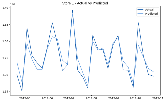
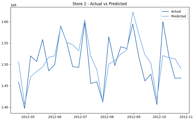
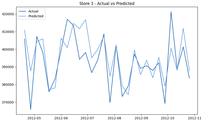
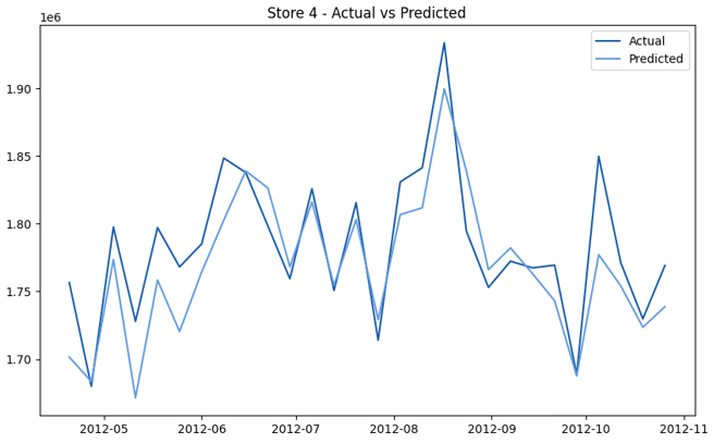
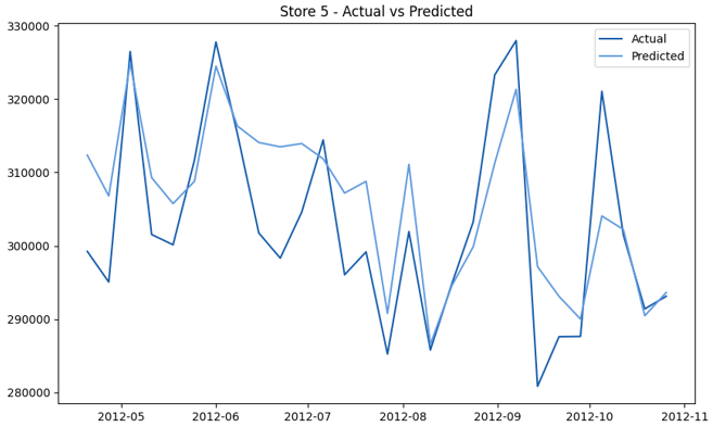
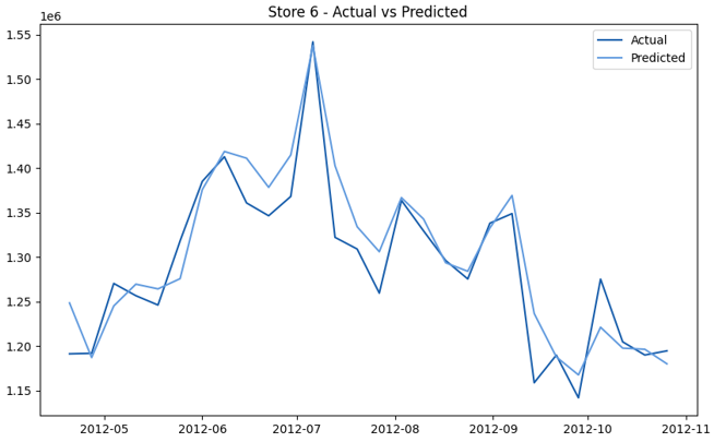
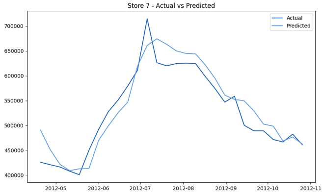
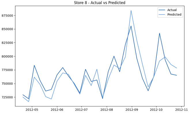
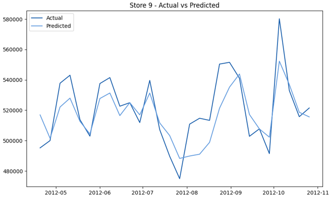
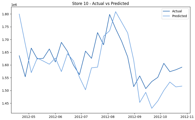
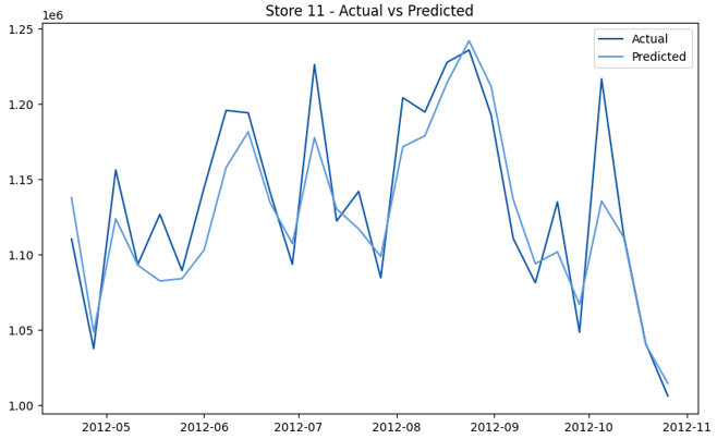
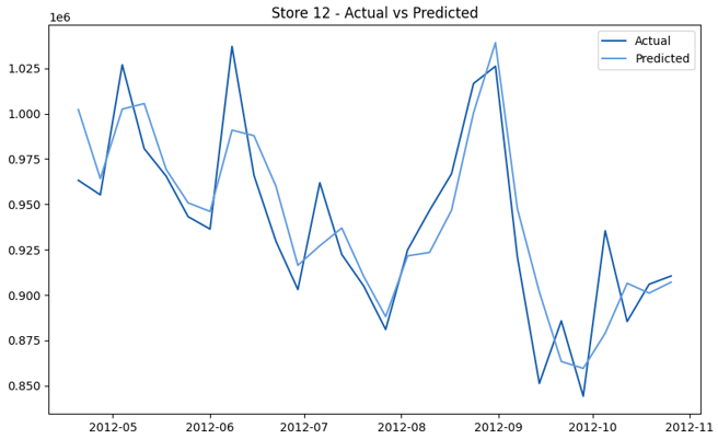
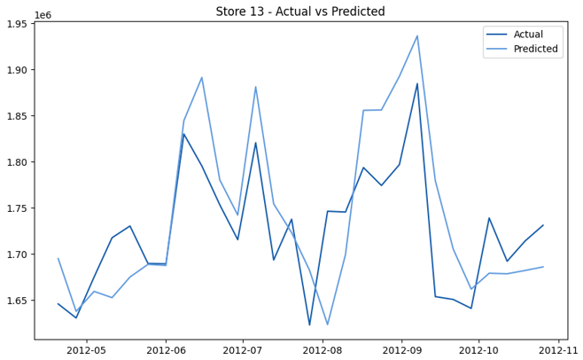
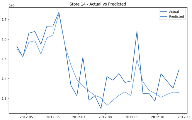
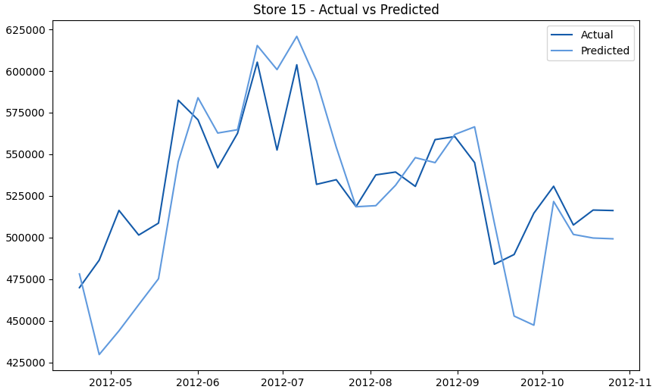
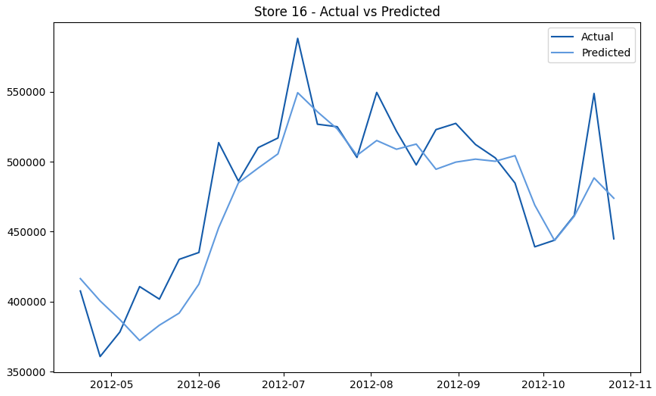
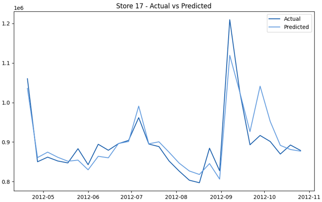
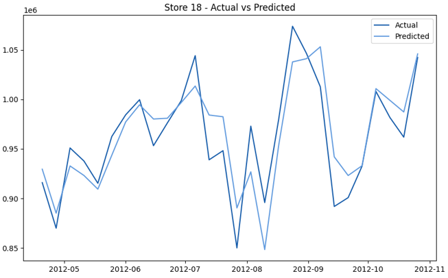
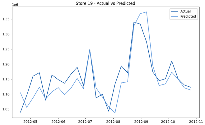
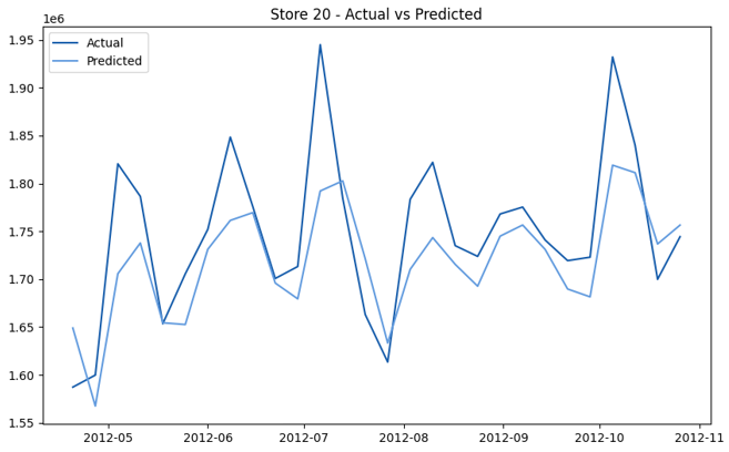
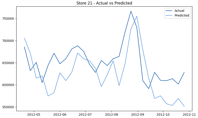
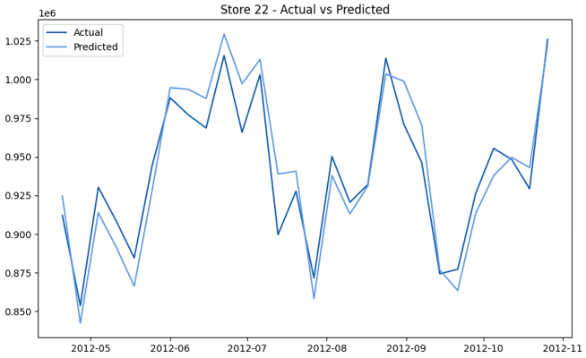
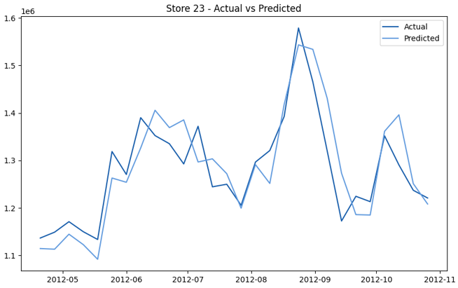
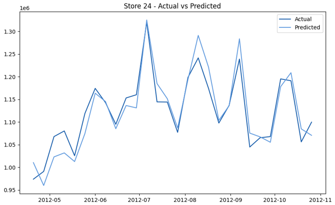
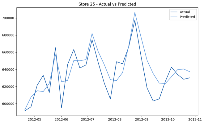
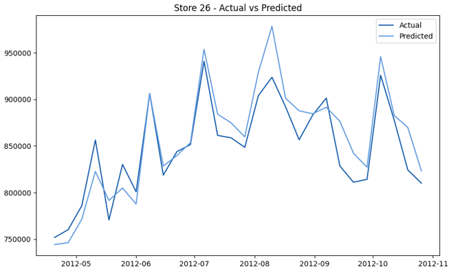
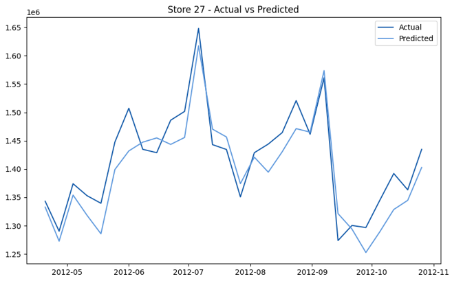
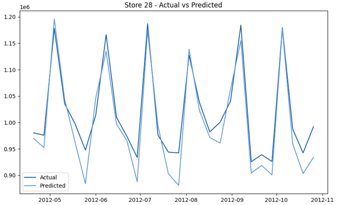
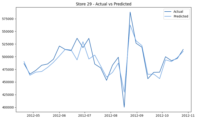
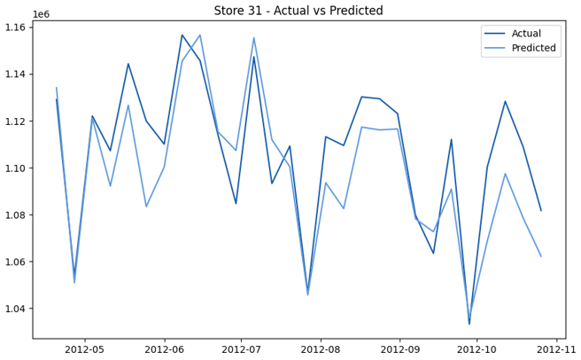
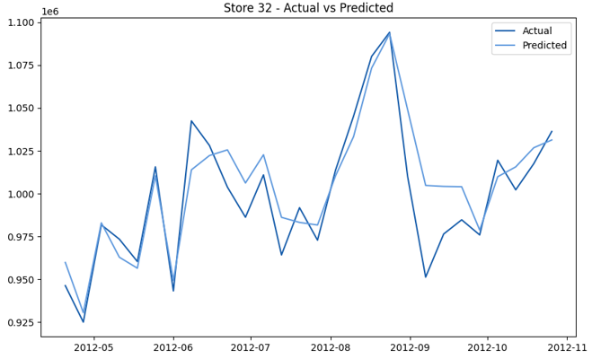
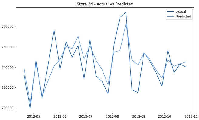
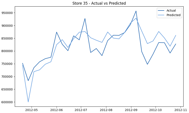
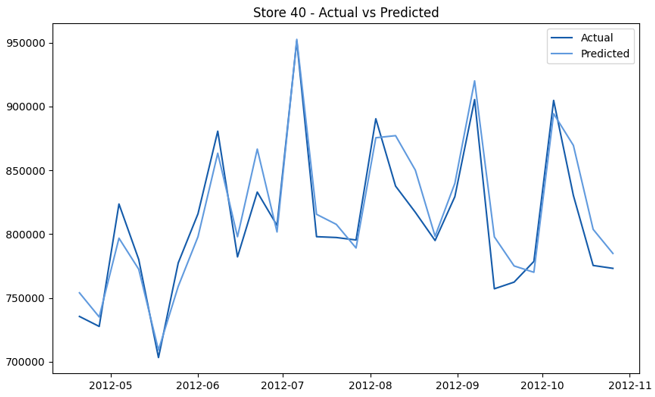
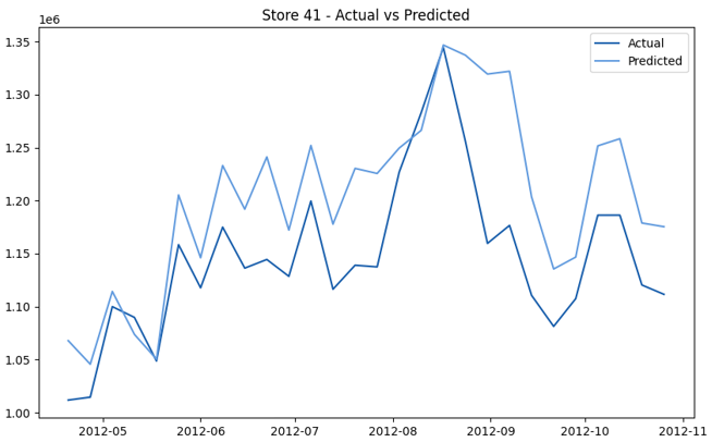
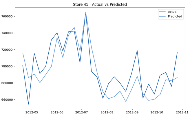
This model demonstrates a substantial reduction in prediction errors and explains over 99\% of the variance in the sales data. These results highlight the superior performance of the hierarchical hybrid approach, marking a significant advancement in accuracy and reliability compared to previous models. The success of this approach underscores the importance of capturing both temporal dependencies and the influence of external factors at a granular level, delivering a highly accurate and reliable sales forecast. Appendix 1 presents the actual vs. predicted final weekly sales forecast for the 45 stores, offering further insights into the model's performance across individual locations.

The results of this study highlight the strengths and limitations of different modeling approaches in forecasting Walmart's weekly sales. Time series and regression models provide a solid baseline but struggle to capture the complexity of retail data, as evidenced by their higher MAE and RMSE values in Figure 14. DL models, particularly the Single Layer LSTM, show marked improvements by capturing long-term dependencies and sequential patterns, resulting in lower error metrics and improved R$^2$ values. However, the hierarchical hybrid model, which forecasts sales at the store level, emerges as the most effective approach, underscoring the importance of granularity in improving forecast accuracy.

Accurate sales forecasting is essential for effective inventory management in large-scale retail operations like Walmart. The findings from this study demonstrate that selecting the right forecasting model is crucial given the complexity and variability of sales data. DL models, such as the Single Layer LSTM and GRU, perform well in capturing long-term trends, making them suitable for general sales predictions. However, neither traditional models nor DL models alone are sufficient to handle sharp demand fluctuations, which are critical for making accurate inventory decisions. The hierarchical hybrid approach offers the most robust solutions for Walmart’s sales forecasting and inventory management. By modeling sales at the individual store level, the hierarchical hybrid model allows for a more precise prediction of inventory needs, resulting in better demand forecasts. This accuracy minimizes excess inventory costs and reduces the risk of stockouts, leading to more efficient inventory management. The hierarchical hybrid model's ability to explain 99\% of the variance in sales data demonstrates its reliability and potential as a key tool in optimizing inventory management across Walmart’s extensive store network.

The findings of this study can be extend beyond forecasting accuracy and offer meaningful implications for data-driven decision-making in retail operations. The proposed hybrid forecasting framework, which integrates time series, regression, and machine learning models within a hierarchical structure, provides highly reliable demand estimates that can be directly embedded into operational, tactical, and strategic decision processes.

At the operational level, improved forecasting accuracy enables more precise inventory control decisions, including replenishment quantity, reorder timing, and safety stock determination. By reducing forecast errors, retailers can lower uncertainty in demand estimation, which in turn minimizes the risk of stockouts and excessive inventory. This supports a transition from reactive to predictive inventory management, allowing retailers to maintain optimal stock levels while reducing holding and shortage costs.

At the tactical level, the model facilitates more effective coordination across the supply chain. Accurate store-level and aggregated forecasts can support distribution planning, warehouse allocation, and workforce scheduling. In addition, the ability of the hybrid approach to capture temporal dynamics and external influences enhances demand visibility, enabling better alignment of promotional strategies and logistics operations with anticipated demand fluctuations. This leads to improved service levels and more efficient resource utilization.

From a strategic perspective, sustained forecasting performance can inform long-term planning and investment decisions. Retailers can leverage consistent demand insights to optimize network design, capacity planning, and supplier engagement strategies. The hierarchical nature of the proposed model further supports multi-level decision-making, ensuring coherence between store-level operations and corporate-level strategies. Over time, this contributes to building a more resilient and data-driven retail ecosystem.

The study also highlights broader managerial and policy implications. Managers can use the proposed framework as a decision-support tool to enhance operational efficiency, reduce costs, and improve customer satisfaction through better product availability. Furthermore, minimizing overstock contributes to reducing waste, aligning inventory management practices with sustainability objectives. The results also underscore the importance of adopting advanced analytics and artificial intelligence in retail systems, encouraging investment in integrated forecasting and enterprise decision-support platforms.

This study aimed to enhance demand forecasting (DF) accuracy by applying various machine learning techniques to Walmart's historical sales data. Key findings highlight the limitations of traditional models in capturing complex retail sales patterns and the improved performance of deep learning models like Single Layer LSTM and GRU in handling long-term dependencies, although these models were computationally intensive. The hierarchical hybrid approach emerged as the top performer, achieving an MAE of 306,361.11, RMSE of 528,096.34, and R$^2$ value of 0.99 successfully modeling sales at both store and aggregate levels by incorporating temporal and external factors.

The contributions include extensive data preparation steps, efficient exploration of over 30 models using AutoML, and the introduction of a hierarchical hybrid model that integrates DL with RF to capture localized patterns alongside broader trends. This approach provides valuable insights for inventory management, enabling tailored, store-level inventory strategies that optimize stock levels and respond effectively to market shifts.

However, the study has limitations: the dataset is outdated and lacks details on online sales, competitor actions, and marketing influences, which limits the models’ ability to capture modern retail dynamics. Additionally, the computational demands of deep learning models and hybrid approaches could pose challenges for resource-constrained retailers.

Future research could incorporate additional external data sources and expand the hierarchical hybrid approach to forecast at more granular levels, such as departments or product categories. Exploring distributed learning methods, like federated learning, could allow individual stores or regions to train models on their specific data, capturing local patterns and nuances more effectively. The insights from these local models can then be aggregated to improve the overall performance of a global model, resulting in more accurate predictions across diverse locations while maintaining the security and confidentiality of sensitive data. These advancements could further improve DF and inventory management, offering retailers actionable insights for more informed decision-making.