From “How to Model a Painting” to the Digital Twin Design of Canvas Paintings
Abstract:
Preventive conservation is conductive to the long-term preservation of works of art. In order to realize the avoidance of damages in advance, risk management as well as foresighted thinking is required. The application of the method of engineering mechanics for preventive conservation is at the very beginning of its development. This article is a contribution to this still very young field. Generally, sensitive artworks combine all properties of complex mechanical structures. Oil paintings on canvas, for instance, are asymmetric, multiple curvilinear structures made of aged anisotropic compound materials with cracks and other damages. Due to their popularity, some artworks travel a lot, and during the exhibition and storage, they are always exposed to shocks and vibrations, therefore the protection of sensitive paintings is a demanding task, the solution of which requires the multidisciplinary cooperation especially in the context of engineering mechanics with its many specializations. The subject of the presented research is an artificial aged painting dummy in the simplest conceivable composition. This paper aims to describe the mechanical behavior of this test object, which is the basic requirement for the development of technological protective measures. The concept of the digital twin, known from Industry 4.0, is used to solve this task. This article focuses on the design of a virtual painting dummy that has the same static and dynamic behavior as the investigated real test object. Therefore, the deflection of the real dummy in lying position as well as the curvature of its standing position without and with dynamic excitations have been measured. The advantage of the analytical and Finite Element Analysis (FEA) models presented are their practicability and quick realizability at fair correlation. The concept presented offers a potential way to assess and finally reduce the risk for original paintings during various transport, exhibition, and storage situations with the help of virtual objects.
1. Introduction
Since museums are operated on a business level [1], the preservation of works of art or the “cultural capital” is regarded as the sovereign task of museums [2]. Consequently, further steps need to be made in terms of risk management and preventive conservation. Following Industry 4.0 methods and adapting to the needs of works of art and the requirements of the cultural heritage sector, the digital twin concept [3] is used in this article as a basis for a predictive risk assessment with the option of developing effective protective measures such as customized backing board constructions [4] and tailormade transport crate solutions [5].
Risk management and the development of protective measure for works of art are fields of the preventive conservation which are systematically explained in the handbook of Waentig et al. [6]. The guide [7] provides a practical guide of risk management of cultural heritage. The application of the concept of digital twin with the methods of engineering mechanics represents a consistent state-of-the-art expansion and science of preventive conservation of works of art and museum objects. Measurement and modeling are central to the application of the digital twin concept. At the later stage, the condition monitoring ensures constant model-updating and the feedback from the simulations with the virtual object in its virtual environment ensures that the real object is preserved sustainably in the long term. The following provides an overview of the state-of-the-art measurements and modeling of mechanical behavior and prediction of responses.
Modeling paintings on textile started in the late 1980s by applying the classical laminate theory [8]. In 2011 and 2013, dissertations on the simulation of the vibration behavior of oil paintings were published independently. While Kracht developed a measurement method to determine high-resolution characteristic vibration modes and frequencies as well as investigated the characterization of nonlinear vibrational behavior [9], Chiriboga focused on modeling the vibrational behavior of canvas using the finite element method [10]. When modeling the material behavior, Chiriboga used the usual mixing rules for compound materials. The modeling basis in both works was Mindlin’s plate theory, whereby Kracht already worked out and considered the importance of taking the prestress into account. Ten years later, in 2021, further experimental studies on the vibration behavior of oil paintings, especially modal nonlinearities, were carried out in the study by Hartlieb [11] and Gao et al. [12].
Due to the importance of pre-stress and pre-strain, paintings on textile are considered as a membrane in the study of Hornig-Klamroth [13]. Hornig-Klamroth concluded that the stiffness of the paint should not be neglected in the modeling. Taking up this advice and based on own experimental experiences, original paintings have been modeled as pre-loaded shells according to Mindlin’s theory with isotropic material behavior adapted to measured characteristic modes and frequencies by a model-updating in the study of Lipp and Kracht [4], [14].
Another important aspect regarding the preservation of works of art is the knowledge about excitation, which is the first “Physical Force” in this article. The acquisition of experimental data during shipment and inhouse-transportation is the subject of many papers. An overview about the research until 2017 is given in the study of Kracht and Kletschkowski [15]. Vibration measurements and reduction measures during construction work are documented in the study by Higgit et al. [16]. In Baseline limits for allowable vibrations for objects [17], limits for allowable vibrations to objects are discussed on base spot tests. A proposal for objectified monitoring of the transport of paintings is made in the study by Heinemann et al. [18].
Vibration behavior, modeling, monitoring, simulation of forced vibrations, and protective measures are elements of the preventive conservation and keys of the digital concept. There is hardly anything else that seems more obvious than the application of the methods of engineering mechanics within the framework of the digital twin concept for the preservation of works of art and museum objects. Although there is a lot of ambition to standardize the terminology across application boundaries, a standard has not been defined yet [19], [20] and the basic concept of digital twin modeling has not been changed since 2002. According to Grieves [3] all elements of the digital twin concept are shown in Figure 1.

The digital twin concept is a further logical development of the model-updating presented in the study of Friswell and Mottershead [21], which was used in the 1990s for model-based parametric system identification [22] for applications like the experimental modal testing [23]. While the acquisition of the static and vibrational behavior of the real object by the measurement method mentioned in the study [9] has well developed, the design of the virtual object is still unclear.
The experimental investigations in the study [9] turned out that the type of the base model (membrane, plate, shell, linear, non-linear) to reproduce the deflection behavior of the real object in the virtual space in out-of plane direction is dependent on the ratio between the bending stiffness and the pretension. The studies in the study [9] also show that the base model must be able to calculate wrinkling, buckling and non-linear vibration behavior depending on the force level of the excitation.
The next step follows in this article is to consider an artificially aged dummy painting in a simple composition. The goal is to design a virtual twin with the same static and dynamic bending behavior as the physical one. Therefore, no base model is excluded from the start. The decision for a base model is made from a questionnaire completed by a conservator, a-priori knowledge about the material behavior gained from tensile testing and results of static and dynamic measurements according to the study [9] as well as detected dominant phenomena. The flow of the design process is demonstrated in the chart of Figure 2.
After collecting all data from the questionnaire, material testing and measurements according to the study [9] in Section 2, first an analytical model based on the consistent plate theory is examined in Section 3.1 of this study. The great advantage of the analytical models is their computational efficiency and mathematical accuracy. However, local characteristics can only be modeled to a limited extent. Numerical Finite Element Analysis (FEA) models can overcome this disadvantage. The investigation to what extent the respective precision and the inaccuracies affect the result is carried out in Section 3.2 and 3.3 in this study. The big challenge here is the handling of the unknown static state of stress due to the pretension. The model-updating and a more detailed model studied in Section 4 and discussed in Section 5 turns out to be the right track. Finally, it is shown that the pretension in combination with the bending stiffness as well as the curvature of the painting play the key role.
2. Experimental Investigations
Regardless of the considered base model, the input parameters are always linked to the geometry, the material properties, and the boundary conditions [24]. Unlike technical objects, the material and the initial pretension of paintings on textile are not designed. The material properties of the natural materials used such as linseed oil, flax fiber and pigments are largely unknown, and are subject to research on their drying and aging process. This is to be considered against the background that the properties of natural materials are widely scattered and the canvas with the paint is deformed in all three spatial directions by the chemical drying process of the paint [9]. Furthermore, material changes and damage such as cracks, tears, craquelure, and delamination are the nature of the deterioration process.
Therefore, the material behavior, and the static deformation of each painting must be determined experimentally. One of the restorers’ tasks is the logging of the paintings’ condition in a condition report [25] which includes, for instance, the mapping of damages, description of the canvas [26], [27], the distortion of the stretcher and the treatment like consolidation, cleaning, and re-tensioning, etc.
The design of the virtual twin of the test object shown in Figure 3 requires the information of the condition and additional information related to the mechanics of the painting. Based on the structure of condition, a questionnaire has been developed and is completed by a conservator. A selection of the results is presented in Section 2.1. Afterwards the industrially glued canvas and the painted canvas of an equivalent painting dummy are documented in Section 2.2.
The static and the vibration behavior of the test object (Figure 3) is determined non-destructively using the Kracht test stand [9]. The results are presented in Section 2.3.
In accordance with study of Kracht [9], with little different materials and making, delamination of the paint test objects has been produced. The dummy making and the documentation of the process have been carried out by Madeleine Vaudremer, a freelance conservator from Utrecht, Netherlands, in the first half of 2020. The non-destructively investigated painting dummy is shown in Figure 3. The cracks and craquelure are documented in Appendix B.
The painting layer system is built up with industrial glue and primer as well as Winsor and Newton Oil Painting alkyd-based primer (2 layers) followed by 3 layers of Zinc white (Mussini 102 series 2, Schmincke) and Cobalt blue light (Mussini 480, series 5, Schmincke). After 6 months of natural drying, the painting dummies have been artificially aged in the climate chamber at BSFV Verpackungsinstitut Hamburg. The two logged climate change cycle series during artificial aging are shown in Figure 4.
The questionnaire of the aged painting dummy has been completed by Daniela Hedinger, a freelance restorer, and conservator from Stuttgart, Germany:
The weight of the test object is 835 g, with the stretcher weighting 595 g. The thickness of the stretcher is 1.7 cm and the width of the bars is 4.3 cm. There is one cross bar in the center of the stretcher, which is made of spruce. The tension of the canvas is in a good condition, which means no wrinkling or buckling effects are visible. The applied textile is characterized according to Rouba [26] and documented according to Lipinski [27]. The parameters are summarized in Appendix A.
The thickness of the painted canvas has been determined with two fixed-distance triangulation lasers facing each other as shown in Figure 5. The lasers and the screen are aligned in such a way that laser beam 1 points normally to the surface of the back of the canvas and laser beam 2, to the front of the canvas. The intersections of the laser beams with the front and back respectively have the same x- and y-coordinates. The reference basis is documented in Figure 3.
Triangular lasers are distance sensors. The fix distance between the lasers is $\mathrm{D}$, while the distance between the back side of the canvas and laser 1 is denoted by $d_1$, and the distance between the front side and laser 2 by $d_2$. The thickness of the painted canvas in the given point is calculated with
$t_{\text {canvas }}=D-\left(d_1+d_2\right)$.
The thickness of the painted canvas was measured at 5 points on each of the blue and white sides. The arithmetic mean of the measured thicknesses for the blue side is 3.3 mm and for the white side, 3.5 mm.
The textile is attached at the tensioning sides of the stretcher using 1 cm long staples. The position and number of staples are marked and documented in Appendix A. No tension garlands are detected.
Destructive tensile tests cannot be carried out on original valuable paintings. Reference values are necessary for a causal model-updating. In the present research, a painting dummy equivalent to the non-destructive investigated one has been cut into strips lengthwise and crosswise. With the help of the tensile testing machine (MTS Tytron 250) from the Chair of Continuum Mechanics and Material Theory, TU Berlin, tensile tests have been carried out on 3 samples of the unpainted and the painted canvas: canvas with industrial glue, canvas with white and blue, weft as well as warp. The experimental set-up is shown in Figure 6.
The resulting averaged stress-strain diagrams are shown in Figure 7, Figure 8 and Figure 9.
A load of approx. 1 N was applied to the test object in the experiment. The effected deformations are so small that linear material behavior can be assumed. Furthermore, the painted canvas is modeled as an isotropic material as this research focused on the development of an easy-to-apply and efficient solution. Therefore, the Young’s modulus is determined by the slope of the tangent to the stress-strain diagram near the origin. The results are:
- Canvas: Incline of the warp tangent line 135 N/mm², Incline of the weft tangent line 2.1 N/mm²,
- White side: Incline of the warp tangent line 145 N/mm², Incline of the weft tangent line 28.7 N/mm²,
- Blue side: Incline of the warp tangent line 29.9 N/mm², Incline of the weft tangent line 340 N/mm².
From the slopes of the tangents, it can be seen that the immense stiffness increases due to the existence of paint.
The investigation of the static displacement field due to gravitation of the standing as well as the lying painting dummy and the measurement of the dynamic displacement field due to dynamic forces of the standing test object have been carried out with a test stand according to Kracht [9]. The two set-ups are shown in Figure 10.
One or three triangular lasers have been used to measure the displacement fields of the painted canvas. The two applied laser configurations are shown in Figure 11.
The motivation of using three lasers is to check experimentally whether unexpected great displacements in in plane-direction occur. The results of all measurements with the three-laser configuration show that the values of the maximum displacement in both plane-directions are 1% of the maximum displacement amplitude in out-of plane direction. Therefore, only the deformations in the much softer out-of plane direction compared to the in the plane-direction are considered further.
The deformations are measured at the frontside of the real canvas at 107x164 positions (107 measurement points in x-direction and 167 measurement points in y-direction). The displacement field of the standing painting loaded by the gravitation field is shown in Figure 12. The measurement data set is evaluated with the software Wolfram Mathematica 12.3.
The two bulges, the lower right corner of the stretcher twisting by 1mm and the overlapping section in the middle of the test object are clearly visible. The displacement field of the lying painting is shown in Figure 13.
The two bulges, the twisted lower right corner of the stretcher and the overlap section in the middle of the test object are still clearly visible. The maximum deformation shown in Figure 13 is approx. 1.34 mm. The investigation of the vibration behavior requires additionally the gravitational field dynamic force to excite the painting. Therefore, the elastically supported stretcher is on the backside connected to an electrodynamic shaker via a force cell and a stinger. The excitation signal is a sinus sweep from 1 to 64 Hz with a time span of 2 s.
Since the nonlinearity check according to Kracht [9] shows a strong dependency on the level of the excitation, the following results are therefore only valid for an excitation amplitude of (1±0.1) N.The characteristic vibration frequencies are identified by picking the peaks of the amplitude frequency response. The amplitude frequency response over all measurements is shown in Figure 14.
The first peak at 6 Hz is affected by the first natural vibration of the easel. The characteristic vibration modes associated to the first characteristic frequencies are shown in Figure 15.
The extremal areas of the measured characteristic eigenmodes are deformed in comparison to the eigenmodes calculated with standard membrane or plate theories presented in the study of Leissa and Qatu [28].
3. Static Deformation of the Lying Painting
This chapter studies the modeling of the deformation field of the lying painting in the earth’s gravitational field. It starts with an analytical solution. Although the analytical theory does not allow any modeling details, it is exact within the model assumptions and serves as a comparison standard for simple examples. Furthermore, the calculation process is very fast.
Since the analytical solution emerges from the consistent plate theory, which in turn is derived from the exact 3D continuum theory, the problem with the finite element method (FEM) here, in particular with volume elements is consequently solved in Section 3.2. On the one hand, these results are validated with the exact solution of the analytical model and, on the other hand, they serve as a comparison standard for the FE-calculations with plate elements in Section 3.3. Since the stiffness matrix is unknown, the stiffness is calculated in all three chapters using the least squares method. The displacement fields thus calculated are compared with the measured ones (Figure 13).
In this Section an analytical model is created for the description of the static behavior of the lying canvas painting. The Young’s modulus is inversely determined by using the analytical model and the experimental data acquired from the lying painting presented in Section 2.3. The quality of the resulting model is evaluated by comparing its deformations with that from the experimental data.
Contrary to the first impulse to model the canvas painting as membrane, according to reference [13] and the findings in Section 2.2, the high bending stiffness due to the existence of paint led to the application of the plate theory. The maximum deformation of the lying canvas with an amount of approximately 1.38 mm (Section 2.3) is smaller compared to the dimensions of the test object. As a result, the painted canvas is assumed to be linear-elastic with only small deformations. Additionally, according to Section 2.1, isotropic material behavior is assumed.
In order to arrive at an analytical solution, the thickness is assumed to be constant all over the plate. Figure 16 shows the plate with its geometrical data $a$ as width, $b$ as length, $h$ as height, $x_i$ as dimensionalized coordinates and $\xi_i=x_i / a$ as dimensionless coordinates.
Moreover, also the surface loads $\vec{g}^{+}$and $\vec{g}^{-}$and the volume load $\vec{f}$ (acting on the volume part $d V$) which initially can point in any arbitrary direction are shown, too. The staples on the edges of the plate (appendix A) prevent the canvas deforming in $x_3-$ and $x_1-$ or $x_2-$ direction. The painting is just loaded by the gravitational field, so the surface loads are zero. The boundary conditions can be summarized as:
and is called "Klemmschneidenlagerung" ("constraint" simply supported). With $\sigma_{i j}$ here the components of the stress tensor and with $u_i$ the components of the displacement vector are introduced. It should be mentioned that when $\xi_1=0,1$, the displacement $u_1$ is zero and when $\xi_2=0, b / a$, the displacement $u_2$ is also zero. The stresses $\sigma_{11}$ and $\sigma_{22}$ are not zero because of the effect of the staples. However, in this Section, these facts are omitted to arrive at an analytical solution. Consequently, the determined Young's modulus is greater than the real one.
According to the assumptions that the canvas painting is linear-elastic and isotropic, the best mechanical model to simulate the deformation of the painted canvas due to its dead weight is the three-dimensional theory of linear elasticity [30]. However, the disadvantage of that theory is that it offers an analytical solution only for some special cases. On the contrary, plate theories have an increased potential for closed-form analytic solutions.
With respect to the above mentioned, the most accurate plate theory is the one which is in accordance with the three-dimensional theory of linear elasticity (linear 3D theory). According to Kienzler and Schneider [31] and Meyer-Coors [32], for the consistent plate theories or original-plate theories this is the case. The latter is even directly derived from the linear 3D theory. Starting point of the derivation are the Neumann-boundary conditions on the upper and lower face of the plate:
The upper index at the stress components indicates that only the even $(e)$ or odd $(O)$ part is considered. The same is valid for the surface loads $g_i$ on the right side. Additionally, the hat-symbol $(\hat{g})$ identifies the dimensionalized quantities and the "+" or "-" sign at the right-upper index indicates the location of the load (e.g. "+" means on the lower side of the plate (cf. Figure 16)). In general, there should be three conditions on each face. But here the six conditions are linear dependent on each other, so only three conditions for both faces are independent. In addition to the Neumann-boundary conditions, (4)-(6) are also the equilibrium conditions:
that are needed to derive the original-plate theories. Here, with $(\bullet)_{, i}$ the derivation with respect to $\xi_i$ is introduced. Next, the displacements in the Eqns. (4)-(9) are substituted by their Taylor series with respect to the thickness coordinate $\xi_3$ :
Subsequently, the modularity of the displacement coefficients is as follows:
which splits the displacement coefficients ${ }^n u_i$ into the so-called displacement-coefficient parts (DCPs) which are inserted in the study by Meyer-Coors [32]. A DCP ${ }^n u_i^p$ has the magnitude $c^p$, where $c=h /(\sqrt{12} a)$ is the so-called plate parameter, which describes the thinness of the plate. Based on the powers of $c$ (magnitude), the Eqns. (4)-(9) are approximated to finally arrive at the original-plate theories. Exemplarily, the steps from above are applied to Eq. (4). It follows:
Here, Hooke's law is applied with $G$ as Shear modulus, $v$ as Poisson's ratio and the two shortcuts $(\bullet)_{,1}=(\bullet)^{\prime}$ and $(\bullet)_{, 2}=(\bullet)^{\bullet}$.
All equations of the magnitude $c^{2N}$ together build the $N_{\text {th}}$-order original-plate theory. The resulting PDE systems can be reduced to one main PDE (only written in the main variable) and severa 1 reduction PDEs (written in the main and the non-main variables). These PDEs are given in the Appendix B in the first and second order. For more details regarding the derivation of the original-plate theories please refer to the study by Kienzler and Schneider [31].
It turns out that the main PDEs (34) and (41) are equivalent to the classical plate theories of Kirchhoff and Reissner, respectively [30]. Therefore, these theories are consistent to the linear 3D theory. This result is not new since justifications of Kirchhoff's and Reissner's plate theories had already been provided by the study of Morgenstern [33] and Paroni et al. [34], respectively. But the advantage of the original-plate theories is that the plate theories in arbitrary order (e.g., 10th order) that are automatically in accordance with the linear 3D theory can be derived. So, if it's necessary, the accuracy of the results can be easily increased by using the third-order theory.
To solve the problem given by the boundary conditions of Section 3.1.1 and the PDEs (31)-(41) (Appendix B), Navier's-double-series solution are applied in the following. Accordingly [35], the ansatz:
for the main variables ${ }^0 u_3^{2 k}$ is used. This ansatz satisfies the boundary conditions (1)-(3) automatically.
The next step is the insertion of (14) into the main PDEs (34) and (41) (Appendix B) to determine the constants $w_{m n}^0$ for the first-order and $w_{m n}^1$ for the second-order theory. Therefore, the applied load is represented by its double-Fourier series. The only load, i.e. the dead weight, is considered as (piecewise) constant volume load ${ }^0 \hat{f}_3=\rho$ g. Here, $\rho$ is the density of the canvas and $g$ is the free-fall acceleration. Since $g$ is a physical constant, only $\rho$ needs to be represented by its double Fourier series:
The constant ρmn can be calculated by the formula:
The different densities of the white (ρW) and blue side (ρB) of the canvas painting can be calculated by:
Besides this, an averaged density $\bar{\rho}$ for both sides can be calculated by simplifying Eq. (17) to:
In the following, both options are expressed by $\rho_{m n} \in\left\{\rho_{m n}^1, \rho_{m n}^2\right\}$.
Now, inserting (14) and (15) into (34), and the following:
is obtained.
It is noted that $\Delta=\frac{\partial^2}{\partial \xi_1^2}+\frac{\partial^2}{\partial \xi_2^2}$ is the Laplacian, $\gamma_{m n}=\sqrt{(m \pi)^2+(n \pi \alpha)^2}, K=\frac{E h^2}{12\left(1-v^2\right)}$ is the plate stiffness and the coefficient comparison is applied. From the second-order theory, it follows:
With the results of (19) and (20), the two main variables:
can be extracted. If these variables are inserted into the reduction PDEs of Appendix B, the non-main variables are the result (cf. Appendix C). With reference to the Eqns. (10) and (11), the complete displacement ansatz for the second-order theory is given by:
For the first-order theory, only the red-colored DCPs are considered. By inserting the main and non-main variables, these displacements can now be calculated.
For the calculation of the Young's modulus, the computer algebra system (CAS) Mathematica $11.3$ is used. First, the experimental data, which represent the distance between the laser and the canvas painting in the form of $x_1, x_2$ and $x_3$ coordinates are imported. In the experiment the canvas painting is suspended, so the boundary points of the data form the rigid frame. This not perfectly flat frame is then averaged to a plane. Finally, the distances between this plane and the experimental data are the $u_3$ deformations of the canvas painting.
Next, the displacement ansatz (23) with the inserted main variables (21) and (22) and the inserted non-main variables (42)-(50) (Appendix C) is transferred to Mathematica. In accordance with Section 2 , the width $a$ equals to $400 \mathrm{~mm}$, the length $b, 600 \mathrm{~mm}$, the total mass $m_T, 0.835 \mathrm{~kg}$, the mass of the frame $m_F, 0.595 \mathrm{~kg}$, the thickness of the blue side $t_B, 3.3 \mathrm{~mm}$ and the thickness of the white side $t_W, 3.5 \mathrm{~mm}$. From these quantities the mass of the canvas painting with $m_P$ equaling to $0.240 \mathrm{~kg}$ is obtained, and the average height $h=3.4 \mathrm{~mm}$, the volume of the canvas painting $V_P=816,0 \mathrm{~mm}^3$ and the average density $\bar{\rho}=294.12 \mathrm{~kg} / \mathrm{m}^3$. For estimating the different densities $\rho_W$ and $\rho_B$, the average density is simply scaled with the help of the ratio between the thicknesses $t_W$ and $t_B$ and the average height, respectively. E.g., $\rho_W=\bar{\rho} \frac{3,5}{3,4}=302.77 \mathrm{~kg} / \mathrm{m}^3$. The density of the blue side then follows, i.e. $\rho_B=285.47 \mathrm{~kg} / \mathrm{m}^3$. Lastly, the free-fall acceleration on earth $g$ is assumed to be $9.81 \mathrm{~m} / \mathrm{s}^2$ and Poisson's ratio $v$ to be 0.3. The value of the Poisson's ratio was chosen based on a numerical pre-study with respect to its influence on the results. It could be concluded the influence of changes of the Poisson's ratio is negligible.
The next step is to apply the function FindFit from Mathematica to determine the unknown Young's modulus in the plate stiffness $K$. This function executes the method of least squares with the analytical and experimental deformation $u_3$. As a result, the Young's modulus is calculated which leads to the smallest error between both data. To assess the quality of the models or configurations, the absolute values of the differences $\left(\Delta u_3\right)$ between the experimental and the analytical deformations with the computed Young's modulus can be determined. Additionally, also the arithmetic mean $\mu$ and the standard deviation $\sigma$ of those differences can be calculated.
In the following five configurations, which are distinguished by the order of the used plate theory, the location of the evaluation of the plate theory $\left(\xi_3=0\right.$ or $\xi_3=h /(2 a)$ ), the consideration of the frame points (to minimize the influence of the not perfectly flat frame) and the two different types of densities (17) and (18) are considered. The results are presented in Table 1.
Model 1 | Model 2 | Model 3 | Model 4 | Model 5 | |
Order | First | First | First | First | Second |
Location $\xi_3$ | 0 | 0 | 0 | $h /(2 a)$ | 0 |
Frame points | Included | Included | Excluded | Included | Included |
Loading | Const. $(\bar{\rho})$ | Var. $\left(\rho_1, \rho_2\right)$ | Var. $\left(\rho_1, \rho_2\right)$ | Var. $\left(\rho_1, \rho_2\right)$ | Const. $(\bar{\rho})$ |
$E[\mathrm{MPa}]$ | 407.50 | 407.46 | 407.45 | 407.43 | 407.45 |
$u_3 \max [\operatorname{mm}]$ | 1.323 | 1.323 | 1.323 | 1.323 | 1.323 |
$\Delta u_{3 \max }[\mathrm{mm}]$ | 1.04 | 1.042 | 1.042 | 1.042 | 1.04 |
$\mu[\mathrm{mm}]$ | 0.149 | 0.149 | 0.143 | 0.149 | 0.149 |
$\sigma[\mathrm{mm}]$ | 0.128 | 0.128 | 0.129 | 0.128 | 0.128 |
Moreover, the maximum displacements of $u_1$ and $u_2$ in terms of model 4 are $u_{1 \max}=0.018 \mathrm{~mm}$ and $u_{2 \max}=0.013 \mathrm{mm}$.
Comparing with the results represented in Table 1 , it can be concluded that none of the modifications (order of theory, location, frame points and loading) has a significant influence on the results:
The Young's modulus varies negligibly. Hence, the value calculated with the second-order theory (model 5 ) is chosen, so that $E$ equals to $407.45 \mathrm{MPa}$. Likewise, the maximum difference between the analytical and experimental data varies only within a small range around $\Delta u_3 \max [\mathrm{mm}]=1.04 \mathrm{~mm}$. The maximum displacement in $x_3$ direction shows no variation and $u_3 \max$ equals to $1.323 \mathrm{~mm}$. For the mean and standard deviation of the difference, the only change is caused by the exclusion of the frame points. As a result, the mean becomes smaller, while the standard deviation gets bigger. However, the amounts of these variations are so small that they are negligible. Therefore, $\mu$ equaling to $0.149 \mathrm{~mm}$ and the standard deviation $\sigma$ being $0.128 \mathrm{~mm}$ are set. Additionally, and in accordance with Section $2.3$, it is mentioned that the displacements $u_1$ and $u_2$ are irrelevant compared with $u_3$.
All in all, the maximum difference $\Delta u_3 \max$ is quite big in relation to $u_3 \max (\approx 79 \%)$. Also, the mean $\mu$ yields about $11 \%$ of $u_3$ max . But as we can see in Figure 17 , the values from above approximately $0.5$ mm originate purely from the two indentations. If these irregularities are omitted, the quality of the model will be better. However, deviations of about $10 \%$ remain. It is concluded that the derived analytical model is recommended to carry out fast rough calculations.
The calculations in Section $3.1$ have shown that the deviations in the out-of plane direction $\left(u_3\right)$ are about $10 \%$ between the measured displacement field and the displacement field calculated with the analytical plate theory for the lying painting under static load in the earth gravitational field. Locally, the absolute difference of displacements is much higher. To verify the quality and quantity of the analytical solution of the plate theory, the calculations should be recalculated using a numerical method, i.e. the finite element method (FEM). It also offers the capabilities of a high level of detail in the modeling of the lying painting, if required. With more detailed FEmodels, and compared with the analytic plate theory model, the deviations of the displacement $u_3$ between measurement and simulation should be further reduced.
The tool to create the Finite Element-models (FE-models) is the commercial FEM software package Abaqus from Dassault Systêmes. The FE-models are created with the preprocessor (and postprocessor) Abaqus/CAE. The implicit solver Abaqus/Standard is used to perform the FE calculations. The evaluation of the results is carried out with Abaqus/CAE, too.
The advantage of Abaqus/CAE is that all modeling and evaluation tasks can be solved by adopting the internal modeling functions based on Python instead of the usual keyboard input which enables the automatization of the model design and result evaluation. This leads to the acceleration and simultaneous error reduction in the parameter studies in this Section. Consequently, in the following the pre-and post-processing is mainly operated using the interface of $\mathrm{Abaqus} / \mathrm{CAE}$ to the programming language Python.
The canvas with its two different painted sections of equal dimension but different thicknesses (white side: $h_{\text {White }}=3.5 \mathrm{~mm}$ and blue side $: h_{\text {Blue }}=3.3 \mathrm{~mm}$, is modeled geometrically in two variants. In the first variant, both sections have the same thickness: the mean of both thicknesses ($h_{\text {White }}=h_{\text {Blue }}=3.4 \mathrm{~mm}$). The first variant is the basis for the FE-models, i.e. model 1 and model 2 and are designed here in this study. These models are created for a comparison with the results calculated with the consistent plate theory (Section 3.1), whose analytical solution is currently only valid for a constant plate thickness.
The second variant is defined by considering the thickness difference between the two sections of the painting. Therefore, a geometric step is applied. This variant in the study is called model step. An overview of the two variants is shown in Figure 18, as mentioned above. In order not to limit the above mentioned modeling freedoms by the FEM, both models are created as 3D volume models, meshed with 3-dimensional finite elements.
The element type used for meshing the volume models is a brick element. The internal code in Abaqus for this type of element is C3D20R. It is a 3D continuum element (C; 3D) with 20 nodes (20) and a reduced gaussian integration (R). Eight nodes are placed in the corners of the element and the remaining twelve nodes are placed in the center of each edge. For description of the element geometry and the deformation of the element a quadratic, iso-parametric polynomial approach is used. Due to the simplified geometry of the models of the two variants, structured rectangular FE meshes have been generated for all. To check the convergence of the solution of the displacement field, the FE models were meshed with different mesh densities in the x-y plane (20x30; 32x48, 48x72) and with one or two element layers. It is shown that meshing with 32x48 elements and one element layer (Figure 18 left) represents a good compromise between accuracy and cost. Thus, in thickness direction, one element layer is applied in model 1 as well as in model 2 (Figure 18 top right). In model Step, a second element layer is added due to the geometric step at the thicker white section (Figure 18 bottom right).
In accordance with Section 2.2 and 3.1, a linear elastic material model is applied and isotropic material behavior is assumed. For this purpose, Hooke’s law implemented in Abaqus is used. Hooke’s law is written in tensor notation as follows:
where, $\sigma_{i j}$ and $\varepsilon_{k l}$ are each second-order tensors, representing the stresses and the strains. $E_{i j k l}$ is the fourth-order elasticity tensor [29].
Due to the isotropic material behavior, only the two material parameters Young's modulus $E$ and Poisson's ratio $v$ are necessary to complete the elasticity tensor and to describe the relationship between stresses and strains. The values for the two parameters are given in Table 2 depending on the different FE-models and their boundary conditions. It should be noted that the identical value for Young's modulus is used for model 1 and model 2 in configuration 1. This inaccuracy emerges from the fact that the geometric models mentioned are modeled simplistically with an average thickness of the painted canvas. The simplification and the effected inaccuracy are conceded to be able to compare results from the FE-simulations with the results from the calculations with the consistent plate theory. There, at the current state, only analytical solutions for constant plate thicknesses $h$ and constant material parameters $E$ and $v$ are known.
The ratio of the Young's moduli is adjusted in configuration 2 of model 2. Considering the plate theory, the correlation of the stiffness of the plate to its thickness leads to the third power. Thus, the ratio of the two Young's moduli for the white and blue section is as follows:
The values for the material parameters and other relevant data for the FE-models are listed in Table 2 . In addition to the description of the material model with its parameters, further information about the material of the canvas is important: the density. As already mentioned in Section 3.1, due to the lack of experimental data, the average density $\rho_{\text {mean }}$ is determined by the ratio of the mass of the painted canvas and its volume. The average density is applied in model 1 and model Step. The inaccuracy of model 1 in the mass distribution that is affected by applying the same thickness at the white and the blue section is corrected in model 2 with:
The next step is to discuss the boundary conditions with the help of Figure 19, which shows an illustration of the canvas with the two areas, one painted in white and one in blue. At four faces of the six ones, the normal vectors $\vec{n}_{\text {face }}$ point in the plane direction of the painting. The red squares at these four faces of the model in Figure 19 represent positions of the staples at the real object. Here, the distances between the staples are equidistant. Ten staples are on each of the short faces and 16 staples are on each of the long faces. The red areas in Figure 19 are $12.5 \mathrm{~mm}$ wide.
The following study includes three variations of the boundary conditions (BC) named A, B and C. The boundary conditions are specified by referring to the displacements of the nodes of the finite elements at the four inplane faces of the painted canvas. The exemplarily listed boundary conditions below are defined for the face outlined in green in Figure 19, which are as follows:
especially a displacement of $+0.15 \mathrm{~mm}$ in the positive direction of the normal unit vector $\vec{n}_{f a c e}$ for the nodes.
The boundary condition $A$ is called "Klemmschneidenlagerung". Only for this boundary condition, the analytical solution of the consistent plate theory presented in Section $3.1$ is valid. For BC B, the nodes in the regions of the staples (red regions) are additionally fixed at their current positions in plane. BC C then is constructed in the same way as BC B. It differs from BC B only in a nonzero displacement of the nodes at the staples. Here, in positive direction of the normal unit vector of the faces in plane (Figure 19). The displaced nodes are then fixed, like at BC B. The values for the prescribed displacements at the short faces are $\left|u_y\right|=0.15 \mathrm{~mm}$ and at the long faces $\left|u_x\right|=0.1 \mathrm{~mm}$. BC C is used in the FE-models to model a prestressed canvas, like the real ones are. The values of the prescribed displacements are estimated from experimental research on canvases [36].
To apply the dead weight of the canvas as load to the FE-models, the Earth's gravity is applied in Abaqus with $\vec{g}=9.81 \cdot(0,0,-1)^{\mathrm{T}}\left[\mathrm{m} \mathrm{s}^{-2}\right]$ (Figure 20). Thus, the design of the individual FE-models is almost completed. At this state, the determination of the inclination of the canvas edges/frame to the plane of the laser measurement system (LMS) is still missing.
Due to inaccuracies in positioning the canvas in front of the LMS and a stretcher, to which the edges of the canvas have been applied, that is not exactly flat, an inclination of the canvas plane to the LMS plane occurred. The correct inclination of the canvas plane is the basis for a meaningful comparison of the nodal displacements computed with the FEM to the acquired values by the LMS. Thus, the inclination of the canvas plane had to be determined mathematically from the measured points at the edges of the canvas.
To calculate the inclination of the canvas plane, which is represented by the normal unit vector in Figure 20 , the function Fit from Numerical Recipes (FORTRAN Version) [37] is applied. Fit calculates a straight line through a set of data points based on the least squares method. Finally, the results of the FE-models were compared with those from the function Fit. The following normal unit vectors are obtained for two variants of the model geometry (Figure 18):
By applying the values of the normal unit vectors (28), the measured and the computed nodal displacements (see Figure 20) are transformed into the deformation direction of the canvas $u_3$. The design of the FE-models is thus completed.
In accordance with Section $2.3$ and 3.1, mainly the nodal displacements $u_3$ (Figure 20) are considered. Furthermore, the parameter $E$ (Young's modulus), unknown for the real object, is determined in the FE-simulations by a parameter optimization using the principle of the least squares method, aiming to obtain the same deformation behavior of the FE-models like the real canvas. The iterative process of the parameter optimization is created with the Function Brent from Numerical Recipes (FORTRAN Version) [37], programmed as Python script and applied to the Python interface of Abaqus.
The deformations in the out-of plane direction are measured at the frontside of the real canvas with one triangulation laser at 107x164 positions in the LMS plane (x-y plane). To compare the measured values with the FE-simulations, these positions of the measurement points are interpolated to the x-y positions of the nodes of a FE-model front with its 32x48 finite elements.
To check the quality of the solutions from the FE-calculations in comparison with those from the analytical consistent plate theory, the difference of the nodal displacements:
for model 2 config. 1 and boundary condition A ("Klemmschneidenlagerung") is determined (further model data can be found in Table 2). The result $\Delta u_3$ is shown in Figure 21. To evaluate the magnitude of the values of the solution $\Delta u_3$, it should be mentioned that the deformation of the canvas $u_3$ is always in the interval $u_3 \in$ $[-0.6,1.6][\mathrm{mm}]$. This is applied to both the measured and the computed data.
The values of $\Delta u_3$ in Figure 21 are larger than three orders of magnitude, which are smaller than the values of the deformation. It is a negligible deviation. This means that the two different calculation methods lead to almost identical results, which was already expected before.
The results of the calculations with FE-model 1, model 2 in config.1 and config. 2, as well as model Step are compared with the measured values of the LMS to evaluate the models and the measurement data. Exemplary, the calculated deformation fields and differences of the deformation fields for the FE-model 2 config. 2 and model Step are shown with colored plots in Figure 22 and Figure 23.
In the first row on the left, the measured displacements, interpolated to the FE nodes, are shown in both figures. Further to the right in each case, the calculated nodal displacements for the three boundary conditions A, B and C explained above in (27) are presented. In each of the second rows, the differences between experiment and FE-simulations of the nodal displacements:
are shown. The legends of the Figure 22 and Figure 23 are valid for all the sub figures. Furthermore, the legends of both Figure 22 and Figure 23 are identical for a better comparability.
The characteristic data applied to the calculations in this Section is listed in Table 2. These are, on the one hand, the material parameters that were required in the FE-simulations such as the thickness of the canvas $h$, the density $\rho$, the Young's modulus $E$ and the Poisson's ratio $v$. On the other hand, there are the statistical data, computed for the results of the FE-simulations. They include the maximum of the nodal displacements of the canvas, measured ($u_{3 \, max \_ exp}$) and calculated ($u_{3 \, max \_ FEM}$). Further, the maximum difference for the nodal displacement between measurement and FE-simulation at a node is denoted by $\Delta u_{3 \, max}$.
Last but not least, the mean value $\mu$ and the standard deviation $\sigma$ for the difference $\Delta u_3$ are calculated and documented in Table 2. In order to achieve a minimum for the least squares for $\Delta u_3$, the Young's modulus was iteratively adjusted to an optimum during several FE-simulations with one FE-model.
If the results of the calculations in the Figure 22 and Figure 23 are compared, taking the data in Table 2 into account, it can be concluded that the differences between the FE-model 1, -model 2 config.1 and config.2 are small. In these models, the data of model Step deviate slightly by larger values for $\Delta u_3$ and thus by an approximate 10% higher than the standard deviation of $\sigma$. This is caused by the geometric step modeled for the white section of the canvas to account for the thickness differences of the white and blue sections of the real canvas.
Comparing the FE-simulations with the measurement, the Figure 22 and Figure 23 show the largest deviation of the nodal displacements $\Delta u_3$ at the positions of the two indentations at the real object. Otherwise, the order of magnitude of the deviations is small, but in relation to the deformations of the real canvas they are significant.
What is interesting is that due to the small deformations of the canvas and the use of the linear theory of elasticity, there are no differences between the calculated displacement fields $u_3$ with boundary conditions B (without prestress) and C (with prestress). This applies to all FE-models with the uniform thickness $h$. Even for the Model Step the deviations are negligible.
If the results of the simulation in the condition $\mathrm{BC} \mathrm{A}$ ("Klemmschneidenlagerung") is compared with the results in other two boundary conditions $B$ and $C$, the better agreement of the maximum nodal displacements from the measurement $u_{3 \max }$ to those of the calculation $u_{3 \, maxFEM}$ is noticeable for $\mathrm{BC} \mathrm{A}$ (see Table 2). This has been the result for all models except for the model Step. Therefore, BC B and C match best.
Model 1 | Model 2 config. 1 | Model 2 config. 2 | Model Step | |
Parameter | Material Data | |||
h [mm] | 3.4 | 3.4 | 3.4 | 3.5 / 3.3 |
ρ [kgm-3] | 294.12 | 302.77 / 285.47 | 302.77 / 285.47 | 294.12 |
E [MPa] (BC A) | 407.45 | 407.45 | 445.51 / 373.42 | 463.28 |
E [MPa] (BC B) | 107.34 | 107.34 | 117.33 / 98.35 | 121.42 |
E [MPa] (BC C) | 107.27 | 107.27 | 117.28 / 98.30 | 122.25 |
v [-] | 0.3 | 0.3 | 0.3 | 0.3 |
Statistics | Boundary Conditions A: | |||
$u_{{3 \max\_expt}}\,\,[\mathrm{mm}]$ | 1.337 | 1.337 | 1.337 | 1.349 |
$u_{{3 \max\_FEM}}\,\,[\mathrm{mm}]$ | 1.322 | 1.322 | 1.328 | 1.167 |
$\Delta u_{3 \max }[\mathrm{mm}]$ | 1.012 | 1.014 | 1.004 | 1.105 |
μ [mm] | 0.027 | 0.027 | 0.027 | -0.009 |
σ [mm] | 0.193 | 0.193 | 0.194 | 0.245 |
Statistics | Boundary Conditions B: | |||
$u_{{3 \max \_expt}}\,\,[\mathrm{mm}]$ | 1.337 | 1.337 | 1.337 | 1.349 |
$u_{{3 \max \_FEM}}\,\,[\mathrm{mm}]$ | 1.500 | 1.500 | 1.503 | 1.333 |
$\Delta u_{3 \max }[\mathrm{mm}]$ | 1.143 | 1.145 | 1.137 | 1.222 |
μ [mm] | 0.094 | 0.094 | 0.094 | 0.046 |
σ [mm] | 0.226 | 0.226 | 0.227 | 0.262 |
Statistics | Boundary Conditions C: | |||
$u_{{3 \max \_expt}}\,\,[\mathrm{mm}]$ | 1.337 | 1.337 | 1.337 | 1.349 |
$u_{{3 \max \_FEM}}\,\,[\mathrm{mm}]$ | 1.501 | 1.501 | 1.503 | 1.344 |
$\Delta u_{3 \max }[\mathrm{mm}]$ | 1.143 | 1.145 | 1.137 | 1.214 |
μ [mm] | 0.094 | 0.094 | 0.094 | 0.046 |
σ [mm] | 0.226 | 0.227 | 0.227 | 0.255 |
…/… $\Leftrightarrow$ white/blue section | ||||
For the optimized value in the Young’s modulus, there are large differences between the “soft” boundary condition A and the “stiffer” boundary conditions B and C for all FE-models. The ratio of the Young’s moduli is $\frac{E_{B C A}}{E_{B C B}}=\frac{E_{B C A}}{E_{B C C}} \approx 3.8$. The extent to which the optimized Young’s modulus corresponds to the reality remains to be clarified.
As a conclusion, it can be said that very similar results are obtained for the same simple modeling of the canvas for the consistent plate theory and the FEM (comparing Table 1 with Table 2). However, compared to the measured values of the deformation of the canvas, the relative deviations of the calculations are significant. For this reason, a more precise description of the deformation behavior of the canvas requires a higher level of detail in the modeling. According to the current state of the consistent plate theory, this can only be achieved with the FEM. With modern FEM software, such as Abaqus here, the limits of modeling are greatly extended. This is the big advantage of the FEM. The disadvantages are the high cost for the rent of such a software and the time (also cost) to spend on such a complex software.
In contrast, the consistent plate theory can provide a cost-efficient solution. If the general equations [31] are known, they can be programmed with a little effort, for example, by the easy-to-learn programming language Python which is freeware. If such a calculation program exists with the possibility to declare the relevant parameters such as the Young’s modulus via variables, it is possible to calculate the deformation behavior for geometrically simply designed canvases with adequate accuracy in a short period of time. Another advantage of the consistent plate theory compared to FEM is the analytical instead of the numerical character. This allows the simple and exact formulation of derivatives, e.g. to determine extreme values in the deformation of the canvas or its location.
In Section 3.1 and 3.2, it is worked out that the calculated values of the deformation of the canvas differ greatly from the measured ones. It is concluded that a more accurate description of the deformation behavior of the canvas requires a higher level of detail in the modeling, which can currently only be achieved with FEM. A higher level of detail of FE-models for simulating the mechanical behavior means perspectively considering the natural curvatures of the painting in the step of geometric modeling. The approximation of thin curved surface structures with solid elements can lead to locking effects that cause large errors [38]. Referring to Bischoff [39] the problem of transverse shear locking does not persist for plate and shell elements according to the Kirchhoff/Love theory. Also using higher order trial functions for solid elements can avoid shear lock effects. However, the computing time is very long compared to using plate or shell elements.
The Kirchhoff/Love theory is suitable when the painted canvas with one layer and the initial state curvatures and deformations in the instantaneous configurations are small compared to other dimensions [28]. Since the painted canvas is only treated as a single-layer model in the context of this article, and referring to Section 2 the necessary requirements are also met, the plate and shell theory of Kirchhoff/Love can be applied.
Looking to the future, the modeling of paintings as a single-layer plate or shell shows a lot of advantages, but the multi-layer modeling is also needed to calculate interlaminar tension and to simulate the effects of delamination. Therefore, the modeling in this Section will be pursued with a theory that takes shear effects into account, which has already been considered in [9] and [10]. Consequently, the shear-flexible plate theory according to Leissa and Qatu [28] is applied. In the study of this Section DSQ and DST element formulations of Batoz [40] are used in the application of the professional software Siemens PLM LMS Samtech SamcefField V 18.
As in the Sections 3.1 and 3.2, the modulus of elasticity is calculated backwards with a model-updating applying the general-purpose design program Siemens PLM Samtech BOSSquattro [41]. The parameters are adjusted in such a way that the maximum deformation of the model corresponds to that measured on the real object. The resulting calculated deformation fields are compared with the measured.
The virtual face with the same main dimensions as the real object is divided in 106 elements in x-direction and 161 elements in y-direction regarding the reference basis shown in Figure 3. Quadrangular elements with four integration points are applied.
In the case, the parameters of the blue and white area are different, and the areas are geometrically modelled as separated faces, which are “merged” to one shell with consistent kinematic transition condition between the faces. Each section of this shell can be assigned a separate model and material behavior. In accordance with Section 2.1 here the painted canvas is assumed as one layer made from an isotropic material with linear material behavior. The different variations of parameter and type of constraints are combined in configurations. The studied configurations are:
Config. 1: One thickness, one Young’s modulus, one density, one Poisson’s ratio ν=0.3 for both areas of the painted canvas, BC A “Klemmschneidenlagerung”, optimization parameter: Young’s modulus,
Config. 2: One thickness, one Young’s modulus, one density, one Poisson’s ratio ν=0.3, BC: painted canvas is fixated at a wooden stretcher, which is modeled as framework with one cross bar. The beams are modeled as line elements with a cross section and material data according to Section 2.1 as well as an isotropic material behavior. The stretcher is clamped at the four corners. Optimization parameter: Young’s modulus,
Config. 3: One thickness, one Poisson’s ratio ν=0.3 for both areas of the painted canvas, but different Young’s Modulus, different densities, BC A “Klemmschneidenlagerung”, optimization parameter: Young’s moduli.
Config. 4: One Poisson’s ratio ν=0.3 for both areas of the painted canvas, but different thickness, different Young’s Modulus, different densities, BC A “Klemmschneidenlagerung”, optimization parameters: Young’s moduli.
The Young’s moduli are parameterized. These variables are assigned to mesh sections in the epilogue of Samcef Fields and imported to Boss quattro as optimization variables.
The present study is evaluated in accordance with the analysis in Section 3.2. The values of the input and output parameters are documented in Table 3. All configurations fulfill the requirements of a linear static analysis. Therefore, the module ASEF of Samcef Field is applied.
Config. 1 | Config. 2 | Config. 3 | Config. 4 | |
Parameter | Material Data | |||
h [mm] | 3.4 | 3.4 | 3.4 | 3.5/3.3 |
ρ [kgm-3] | 294.12 | 294.12 | 302.77 / 285.47 | 302.77 / 285.47 |
E [MPa] | 404.54 | 124.12 | 406.76 / 402.74 | 408.44 / 404.40 |
v [-] | 0.3 | 0.3 | 0.3 | 0.3 |
Statistics | “Klemmschneidenlagerung” | |||
$u_{{3 \max }_{\,\,expt}}\,\,[\mathrm{mm}]$ | 1.337 | 1.337 | 1.337 | 1.337 |
$u_{{3 \max }_{\,\,FEM}}\,\,[\mathrm{mm}]$ | 1.337 | 1.337 | 1.337 | 1.338 |
…/… $\Leftrightarrow$ white/blue section | ||||
The differences between the measured and the calculated displacement field of the four configurations are shown in Figure 24.
Both the qualitative appearance of the difference fields and the values are very similar to the results shown in Figures 22 and 23 bottom lines. The extremes are noticeable due to the two indentations, the distorted stretcher especially the lower right corner (referring to Figure 3), the horizontal lines in the center of the canvas and the vertical stripes in the middle of the two edges as well as in the center of the painting.
Using the plate instead of the volume elements does not cause any change in the quality of the results. The differences between the calculated and measured displacement field have remained the same. However, this also means that modeling the mechanical behavior of the painted canvas with shell elements is just as legitimate as modeling it with volume elements. This knowledge also serves to increase the detail of the modeling based on shell elements.
4. Virtual Painting Design
The extremes of the field deviations between the measured and calculated displacement fields in Figure 24 show similarities to Figure 12 which is the deformation field of the standing real object. Since 1.) the load acts on the standing painting almost exclusively in the inplane direction and 2.) neither in Section 2.1 nor in Section 2.3, is wrinkle or buckling behavior determined. It can be assumed that the deformation field in Figure 12 is the initial configuration in the out-of plane direction of the considered problem, the deformation of the lying painting.
If this initial configuration is assumed to be the basic deformation field of the painted canvas (before loaded in out-of plane direction by the gravitation), this is contained in the measured deformation field of the lying canvas (Figure 13). Since the initial deformation is not included in the calculation models, it must be subtracted from the measured deformation field of the lying test object. The corrected measured deformation field of the lying painted canvas is shown in Figure 25.
The corrected displacement field shows the characteristics of a lying canvas under its dead weight as expected. Obviously, the deviation of the displacement field of the lying painting from the expected is affected by the initial state of displacement caused by the natural deformation of the painting and the distortion of the stretcher. The correction of the displacement field also reveals a new value for the maximum displacement of 1.6 mm instead of the previously considered 1.34 mm.
Consequently, the result in Figure 24 needs to be corrected, too. Consequently, the difference between the corrected measurement result and the in Section 3.3 calculated displacement fields is to be generated. The result is shown in Figure 26.
The values, especially the distance between the minimum and maximum, are smaller as expected.
Beside this positive finding, the plots in Figure 26 demonstrate the consequence that in contrast to Section 3.1 and 3.2, the uneven positioning of the painting dummy caused by the suspension (Figure 10 right) is not corrected in this Section. This means that the displacement fields include a rotation around the diagonal from the top white to the bottom blue corner (Figure 3).
Additionally, in the 3D point plot of Figure 25, grooves appear particularly clearly at the points where the canvas is attached to the stretcher frame with the help of staples. Furthermore, as in Section 3.1.1, the calculated Young’s modulus for model 2 that supports the canvas with a wooden stretcher (Table 4) is much smaller compared to other examples. The decrease of the value for the Young’s modulus is also effected by boundary condition B and C in Section 3.2 (Table 2). These boundary conditions respect the clamping with staples and the prescribed displacement at the staples’ position. The pre-stretching of the canvas and the resulting pre-tension has a share in the stiffness matrix, as with the loading of a disc. The pre-strain leads to a coupling problem between the disc and the plate [35].
As a conclusion, the position of the staples and a prescribed displacement of the canvas at these points need to be considered in a more detailed model. The position of the staples is documented in Appendix A, but there are no values for the pre-tension or pre-stretching of the canvas. The only clue is the fact in Section 2.1 that there are no tension garlands, i.e. the pre-stretching of the canvas must be small. Since there are no exact values, the pre-strain is included as the optimization parameters “prescribed displacements” in the model update. A further level of modeling depth relates to the curvature, that is the initial field of deformation of the standing painting. Referring to equation 7.8 on p. 278 in Vibrations of Continuous Systems [28], the curvature influences the stiffness of the shell, too.
In accordance with Sections 2.1 and 3, the painted canvas is assumed as one layer made from an isotropic material with linear material behavior. The studied configurations are:
Config. 5: Even rectangular face, one thickness, one Young’s modulus, one density, one Poisson’s ratio ν=0.3 for both areas of the painted canvas, boundary condition C, optimization parameter: Young’s modulus, prescribed displacements in x- and y-direction,
Config. 6: Even rectangular face, one Poisson’s ratio ν=0.3 for both areas of the painted canvas, but different thicknesses, different Young’s Moduli, different densities for each section, boundary condition C, optimization parameters: Young’s moduli, prescribed displacements in x- and y-direction,
Config. 7: Initial deformation field of standing painting (Figure 12), one Poisson’s ratio ν=0.3 for both areas of the painted canvas, but different thicknesses, different Young’s Moduli, different densities for each section, boundary condition C, optimization parameters: Young’s moduli, prescribed displacements in x- and y-direction.
Shallow shell formulations provide for the consideration of the pretension and the curvature [28]. Therefore, in the study of this Section shell element formulations of Hughes [42] are used in the application of the professional software Siemens PLM LMS Samtech SamcefField V 18, especially the modules Mecano.
The virtual face in config. 5 and 6 has the same main dimensions as the real object. According to Section 2.3 the virtual face is divided in 106 elements in x-direction and 161 elements in y-direction, regarding the reference basis shown in Figure 3. Quadrangular and triangular elements are applied.
Instead of designing a geometry model, in config. 7 the mesh with quadrangular elements is directly generated with the program Wolfram Mathematica 12.3. In accordance with the Bacon programming language a dat-file containing the table with the x and y coordinates of the mesh entities and the corresponding measured displacement in out-of plane direction of the standing painting is generated and imported to SamcefField.
In all configurations, the edges of the virtual surface or the imported mesh are divided into sections to define the positions of the staples. The points between two edge sections are each already automatically meshed. The boundary condition A (“Klemmschneidenlagerung”) is applied to the edge sections between the staple points, while the constraints of the points are the prescribed displacements in in plane direction normal to the edge. This procedure is advantageous compared to vertices that are fixed to the virtual face. The variant with the vertices leads to numerical instabilities.
In order to respect nonlinearities effected by the pretension and the considered initial curvature of the standing painted canvas, the implicit nonlinear solver of the module Mecano is used. For this purpose, the acceleration g=9.81 m/s² is applied to the models in configuration 5 as constant load and in the configurations 6 and 7 the linearly increasing load over time, which has reached the value g=9.81 m/s² at t=0.5 s. Then, the time integration between 0≤t≤1 s is carried out.
The model-updating processes are operated with the general-purpose design program Siemens PLM Samtech BOSSquattro. The target is the maximum deformation of 1.6 mm in z-direction (Figure 3) according to the corrected measured displacement field of the lying painting (Figure 25). Depending on the configuration, the variables to be adjusted are the Young’s moduli and/or the prescribed displacements at the staples’ points. For the Model-Updating, definition ranges for the optimization variables must be specified. These are listed in Table 4.
Young’ modulus (white area) | Young’ modulus (blue area) | Presscr. displ. x-direction | Presscr. displ. y-direction | |
Lower bound | 20 MPa | 20 MPa | 0.01 mm | 0.005 mm |
Upper bound | 145 MPa | 340 MPa | 1 mm | 0.5 mm |
The values for the Young’s moduli are based on the tangent slopes to the stress-strain graphs (Section 2.2), for the prescribed displacements on the fact that no tension garlands are visible (Section 2.1). The values for the prescribed displacements in the x-direction are greater than those in the y-direction because the canvas was first stretched over the two long sides of the stretcher (along the y-direction according to Figure 3). The main stress is therefore orthogonal, which means in the x-direction.
The final set of values of each configuration and the definition of the direction of the prescribed displacements are documented in Table 5.
Table 5 shows that different values are permitted for the prescribed displacement per edge. Along the edges, the prescribed displacement is assumed to be constant. The algebraic sign rule of the prescribed displacements is defined in the figure of Table 5.
The difference displacement fields resulting from the corrected measured displacement field of the lying painting (Figure 25) and the calculated displacement field of config. 5 to 7 with the final sets of data listed in Table 6 are shown in Figure 27.
It is noted that the displacement fields shown in Figure 27 are greatly different from those of the configurations in Figure 26. This means that the parameters pre-strain and curvature have a comparatively large influence on the local deformations.
Since the displacement fields shown in Figure 27 include a rotation around the diagonal from the top white to the bottom blue corner (Figure 3), ideally, the corners normal to that diagonal have opposite extreme values, while the displacement of this diagonal is ZERO (turquoise). Config. 7, parameter set 1, meets these requirements best.
Config. 5 | Config. 6 | Config. 7 | 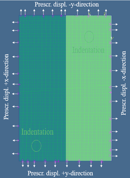 | |
h [mm] | 3.4 | 3.5 / 3.3 | 3.5 / 3.3 | |
ρ [kgm-3] | 294.12 | 302.77 / 285.47 | 302.77 / 285.47 | |
E [MPa] | 26.68 | 24.90 / 20.75 | 34.6 / 20.33 | |
v [-] | 0.3 | 0.3 | 0.3 | |
Prescr. displ. +x-direc. [mm] | 0.3375 | 0.4150 | 0.359 | |
Prescr. displ.-x-direc. [mm] | -0.3394 | -0.4150 | -0.35 | |
Prescr. displ. +y-direc. [mm] | 0.2123 | 0.2078 | 0.29 | |
Prescr. displ.-y-direc. [mm] | -0.2124 | -0.2078 | -0.095 | |
$u_{{3 \max }_{\,\,expt}}\,\,[\mathrm{mm}]$ | 1.6 | 1.6 | 1.6 | |
$u_{{3 \max }_{\,\,FEM}}\,\,[\mathrm{mm}]$ | 1.6 | 1.6 | 1.61 | |
1st natural frequency [Hz] | 15.38 | 15.27 | 15.37 | |
…/… $\Leftrightarrow$ white/blue section | ||||
The static quantities according to Table 3, mean, root of the mean of the squares, variance and standard deviation, are shown in Figure 28. Values are calculated either per column (left) or per row (right). This can be seen from the abscissa values in the diagrams. The statistic values are calculated for 106 columns and 161 rows.
Overall, it can be stated that the difference fields calculated in rows vary much more than those evaluated in columns. The diagrams show that configuration 7 has the smallest mean values in the difference field in both the column and row directions. However, configuration 5 has the smallest standard deviations and variances. The result should be further improved. To be continued, the most promising base modeling, that is, the one considering configuration 7 will be introduced.
One possibility of reducing the magnitude of the difference field is to further adapt the model to the measurements. On the one hand, this can be achieved via the parameter values and, on the other hand, via the model itself and the considered parameters therein (the type of dependencies, the material model, etc.). However, the basic idea is always the adjustment of the measurement data.
In these studies, in addition to the static deflection of the standing and lying painting due to its dead weight, the characteristic vibration modes and vibration frequencies of the standing painting are determined from the response of the test object to a sine sweep excitation with an amplitude in the frequency ranging from 1 to 64 Hz. The reason for this is that further indirect knowledge about the required stiffness matrix can be generated by including the dynamic behavior.
The first natural frequency of the configurations 5 to 7 is documented in Table 6. The calculated values between 15.27 Hz and 15.38 Hz are 1.5 times higher than the measured first characteristic frequency in the amount of 10 Hz (Figure 15). Further measured characteristic vibration frequencies and those with config 7/parameter set 1 are listed in Table 6.
No. | 1 | 2 | 3 | 4 | 5 | 6 | 7 |
Measurement | 10.0 Hz | 12.0 Hz | 16.5 Hz | 20.0 Hz | 27.5 Hz | 32.0 Hz | 34.0 Hz |
FEA-calc. | 15.4 Hz | 20.4 Hz | 27.9 Hz | 30.1 Hz | 34.3 Hz | 37.9 Hz | 40.9 Hz |
No. | 8 | 9 | 10 | 11 | 12 | 13 | 14 |
Measurement | 39.0 Hz | 44.0 Hz | 57.0 Hz | 59.5 Hz | 63.5 Hz | n. m. | n. m. |
FEA-calc. | 48.8 Hz | 49.9 Hz | 50.6 Hz | 52.9 Hz | 59.1 Hz | 63.0 Hz | 64.1 Hz |
No. | 15 | 16 | 17 | 18 | 19 | 20 | 21 |
Measurement | n. m. | n. m. | n. m. | n. m. | n. m. | n. m. | n. m. |
FEA-calc. | 68.2 Hz | 73.0 Hz | 77.0 Hz | 78.4 Hz | 80.4 Hz | 83.3 Hz | 92.1 Hz |
The large deviation of the calculated values from the measured ones runs through the entire frequency range from 1 Hz to about 100 Hz. The vibration modes associated with the characteristic frequencies highlighted in gray are shown in Figure 29 and Figure 30. When comparing the vibration modes, it should be noted that $w_{M E A S_i}$ results from the distance measurement perpendicular to the canvas plane, with the laser beam hitting the painting surface at an angle deviating from 90 degrees due to the imperfect suspension and the distortion of the frame. In addition, there are deviations caused by the roughness of the painting’s surface. Therefore, also the calculated displacement fields in x- and y-direction are shown in the following Figure 29 and Figure 30.
Additionally, the deformations in the x- and y-directions are relevant with 10% of the deformation in the z-direction for the characteristic higher-order vibration modes.
The comparison of the measured and calculated modes shows that there is agreement in principle with regard to the number and position of the extremes. But there are deviations in the form of the extrema.
It is now up to us to discuss whether these deviations are relevant and if so, where they come from and how they are likely to be remedied.
5. Discussion
Both the characteristic frequencies and the associated vibration modes show large deviations. These deviations need to be minimized. The fact is that there are many influencing parameters and great uncertainties in their determination. An optimum is an optimum the specific search process and depends for instance on the starting value. Another parameter set, which also causes 1.6 mm static maximum deformation, is listed in Table 7. The characteristic vibration modes that are associated with the frequencies from Figure 29 and Figure 30 and calculated with parameter set 2 are shown in Figure 31 and Figure 32.
Config. 7 | ||
Parameter set | 1 (as in Table 6) | 2 |
h [mm] | 3.5 / 3.3 | 3.5 / 3.3 |
ρ [kgm-3] | 302.77 / 285.47 | 302.77 / 285.47 |
E [MPa] | 34.6 / 20.33 | 42.2 / 12.5 |
v [-] | 0.3 | 0.3 |
Prescr. displ. +x-direc. [mm] | 0.359 | 0.53 |
Prescr. displ.-x-direc. [mm] | -0.35 | -0.43 |
Prescr. displ. +y-direc. [mm] | 0.29 | 0.21 |
Prescr. displ.-y-direc. [mm] | -0.095 | -0.12 |
$u_{{3 \max }_{\,\,expt}}\,\,[\mathrm{mm}]$ | 1.6 | 1.6 |
$u_{{3 \max }_{\,\,FEM}}\,\,[\mathrm{mm}]$ | 1.61 | 1.61 |
1st natural frequency [Hz] | 15.37 | 15.37 |
…/… $\Leftrightarrow$ white/blue section | ||
Both exemplary eigenmodes are much more like the measured deflection shapes than those of parameter set 1 (Figure 29 and Figure 30) as well as the associated vibration frequencies are also closer to the corresponding measured frequencies. The reason for this is just the new parameter set, which is listed in Table 7.
The difference between the Young’s moduli and the values of the prescribed displacement of parameter set 2 is much greater than that between the Young’s moduli and the values of the prescribed displacement of parameter set 1. This leads to the conclusion that the characteristic vibration modes are strongly dependent on the pre-strain of the canvas. Furthermore, it can be concluded that if the characteristic vibration mode is identical to the measured, the associated characteristic frequency is correct. An extended model-updating can be derived from this.
6. Conclusions
Paintings on textile in museums are subject to the principle of preventive conservation. In order to prevent damage caused by physical, and in particular, mechanical forces in advance, methods from engineering mechanics are adopted in this article as part of the concept of the digital twin. The goal of this paper is to develop a virtual object that has the same static properties as the real painting dummy examined. Due to the lack of knowledge about pre-strain and undeveloped material models, the stiffness matrix is unknown.
With an analytical solution based on the consistent plate theory, the deformation fields can be calculated efficiently depending on various parameters, but the sought Young’s modulus is far too high because the pre-strains cannot be considered.
A study with the volume elements has shown that the FEM can figure out solutions that are almost as exact as analytical models. Although pre-stretching of the canvas is considered, the finding follows that further modeling depth is necessary.
In order to avoid numerical errors in the modeling, it is shown in a further step that the modeling with plate and shell elements is also adequate. The studies with shell elements also show that both the initial static deformation of the painted canvas and the location of the pre-stretched areas of the textile must be taken into account. Satisfactory results are obtained with these details, but it turns out that the characteristic frequencies are too high, and the details of the associated vibration modes do not match those measured. It is shown that with more than one set of parameters for Young’s modulus and pre-strain the finding follows that the measured maximum displacement of the lying painting can be calculated. The calculated parameter sets based on the model-updating aimed to reproduce the maximum deflection of the canvas depend on the initial values. However, it could be shown that if, in addition to the maximum deformation of the painting, the congruence of characteristic vibration modes is required, the associated characteristic vibration frequencies are also approximated to the measured ones. This leads to an extended model-update.
Whether this procedure is sufficient to design a virtual twin must be examined in subsequent scientific work. If this is not the case, the model must be built in detail and also in a more complex manner, considering more precise material models, more detailed pre-strain, more precise two-dimensional determination of the painting in terms of its thickness and nonlinearities.
Kerstin Kracht was the professor at the Faculty of Engineering Mechanics and Structural Mechanics of the University of Bremen in the period from 2021 to 2022 and the visiting professor for the ‘Mechanics of Works of Art and Museums’ Object at the Department of Continuum Mechanics and Material Theory at the TU Berlin in the period from 2020 to 2022. Her profession is in the Vibration Technology and the Continuum Mechanics using mainly PLM LMS Samtech Samcef Field V 18 and Boss Quattro. Her passion lies in the preservation of historical artistic works.
Michael Meyer-Coors was a research associate in the period from 2015 to 2022 with the Falculty of Engineering Mechanics and Structural Mechanics of the University of Bremen. His main research field was the consistent approximation of the three-dimensional theory of linear elasticity (e.g., plates, discs, beams). In 2022, he finished his PhD-thesis with the title “On the development and mathematical justification of consistent-plate theories of any approximation order”.
Roland Schröder has been a scientific and technical associate since 1994 at the Falculty of Engineering Mechanics and Structural Mechanics of the University of Bremen. His main tasks are the programming of numerical models in e.g. Python and the implementation in Abaqus in fields like material modelling and fracture mechanics. He is also co-author of textbooks in Strength of Materials.
The data used to support the findings of this study are available from the corresponding author upon request.
The authors declare that they have no conflicts of interest.
A Questionnaire
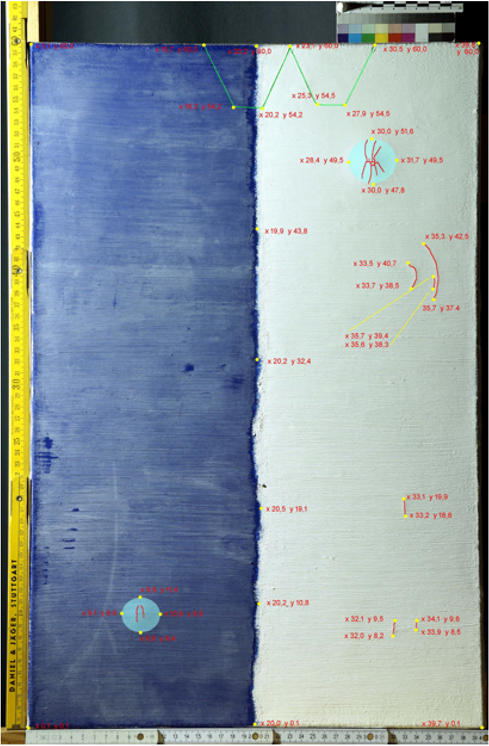
Documentation of cracks and craquelure of the test object
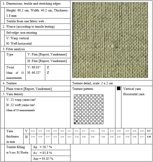
Analysis of structure of the test object canvas
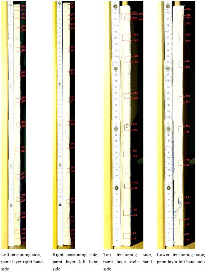
Position and number of staples
B Main and reduction PDEs
For the first-order original-plate theory, we obtain the reduction PDEs
${ }^1 u_1^0=-\left({ }_0^0 u_3^0\right)^{\prime}$, (31)
${}^1 u_2^0=-\left({}^0 u_3^0\right)^{\bullet}$, (32)
${ }^2 u_3^0=\frac{v}{2(1-v)} \Delta^0 u_3^0$ (33)
and the main PDE
$\mathrm{K} \Delta \Delta_{}^0 u_3^0=\mathrm{a}^3\left(h^0 \hat{f}_3+2 \hat{\mathrm{g}}_3^{\mathrm{e}}+\frac{h}{a}\left(\left(\hat{g}_1^{\mathrm{o+}}\right)^{\prime}+\left(\hat{g}_2^{\mathrm{o+}}\right)^{\bullet}\right)\right)$. (34)
For the second-order original-plate theory, we obtain the reduction PDEs
${ }^1 u_1^2=g_1^{o+}-\left({}^0 u_3^2\right)^{\prime}-\frac{3}{1-v} \mathrm{c}^2\left(\Delta^0 u_3^0\right)^{\prime}$, (35)
${ }^1 u_2^2=g_2^{o+}-\left({}^0 u_3^2\right)^{\bullet}-\frac{3}{1-v} \mathrm{c}^2\left(\Delta^0 u_3^0\right)^{\bullet}$, (36)
${}^2 u_3^2=\frac{v}{2(1-v)} \Delta^0 u_3^2+\frac{1+4 v}{4(1-v)^2} c^2 \Delta \Delta^0 u_3^0+\frac{1}{8(1-v)}\left(\left(g_1^{o+}\right)^{\prime}+\left(g_2^{o+}\right)^{\bullet}+2 \frac{a}{h} g_3^{e+}\right)$ (37)
${}^3 u_1^0=\frac{1}{6} \frac{2-v}{(1-v)}\left(\Delta^0 u_3^0\right)^{\prime}$ (38)
${}^3 u_2^0=\frac{1}{6} \frac{2-v}{(1-v)}\left(\Delta^0 u_3^0\right)^{\bullet}$ (39)
${}^4 u_3^0=\frac{1}{24} \frac{1+v}{(1-v)}\Delta\Delta^0 u_3^0$ (40)
and the main PDE:
$\mathrm{K} \Delta \Delta_{}^0 u_3^2=\mathrm{a}^3 \left( -\frac{3}{5} \frac{(8-3 v)}{(1-v)} c^2 \Delta \hat{\mathrm{g}}_3^{\mathrm{e}+}+c^2 h\left(\left({}^1\hat{f}_1\right)^{\prime}+\left({}^1\hat{f}_2\right)^{\bullet}\right)+c^2 h^2 \hat{f}_3 -\frac{1}{10} \frac{(4+v)}{(1-v)} c^2 \frac{h}{a}\left(\left(\Delta \hat{g}_1^{\mathrm{o+}}\right)^{\prime}+\left(\Delta \hat{g}_2^{\circ+}\right)^{\bullet}\right)-\frac{1}{10} \frac{(24+v)}{(1-v)} c^2 h \Delta^0 \hat{f}_3\right)$ (41)
C Solutions of the reduction PDEs
For the first-order original-plate theory, we obtain the reduction PDEs
${}^1u_1^0=-\frac{h a^3 g}{K} \sum_{m, n=1}^{\infty}(m \pi) \frac{\rho_{m n}}{\gamma_{m n}^4} \cos \left(m \pi \xi_1\right) \sin \left(n \pi \alpha \xi_2\right)$, (42)
${}^1u_1^0=-\frac{h a^3 g}{K} \sum_{m, n=1}^{\infty}(n \pi \alpha) \frac{\rho_{m n}}{\gamma_{m n}^4} \sin \left(m \pi \xi_1\right) \cos \left(n \pi \alpha \xi_2\right)$, (43)
${ }^2 u_3^0=-\frac{v}{2(1-v)} \frac{h a^3 g}{K} \sum_{m, n=1}^{\infty} \frac{\rho_{m n}}{\gamma_{m n}^2} \sin \left(m \pi \xi_1\right) \sin \left(n \pi \alpha \xi_2\right)$. (44)
For the second-order original-plate theory, we obtain the reduction PDEs
${ }^1 u_1^2=\frac{1}{10} \frac{(6-v)}{(1-v)} \frac{h a^3 c^2 g}{K} \sum_{m, n=1}^{\infty}(m \pi) \frac{\rho_{m n}}{\gamma_{m n}^2} \cos \left(m \pi \xi_1\right) \sin \left(n \pi \alpha \xi_2\right)$, (45)
${}^1u_2^2=\frac{1}{10} \frac{(6-v)}{(1-v)} \frac{h a^3 c^2 g}{K} \sum_{m, n=1}^{\infty}(n \pi \alpha) \frac{\rho_{m n}}{\gamma_{m n}^2} \sin \left(m \pi \xi_1\right) \cos \left(n \pi \alpha \xi_2\right)$, (46)
${ }^2 u_3^2=\frac{1}{20} \frac{(5+v)}{(1-v)} \frac{h a^3 c^2 g}{K} \sum_{m, n=1}^{\infty} \rho_{m n} \sin \left(m \pi \xi_1\right) \sin \left(n \pi \alpha \xi_2\right)$, (47)
${ }^3 u_1^0=-\frac{1}{6} \frac{(2-v)}{(1-v)} \frac{h a^3 g}{K} \sum_{m, n=1}^{\infty}(m \pi) \frac{\rho_{m n}}{\gamma_{m n}^2} \cos \left(m \pi \xi_1\right) \sin \left(n \pi \alpha \xi_2\right)$, (48)
${ }^3 u_2^0=-\frac{1}{6} \frac{(2-v)}{(1-v)} \frac{h a^3 g}{K} \sum_{m, n=1}^{\infty}(n \pi \alpha) \frac{\rho_{m n}}{\gamma_{m n}^2} \sin \left(m \pi \xi_1\right) \cos \left(n \pi \alpha \xi_2\right)$, (49)
${}^4 u_3^0=-\frac{1}{24} \frac{(1+v)}{(1-v)} \frac{h a^3 g}{K} \sum_{m, n=1}^{\infty} \rho_{m n} \sin \left(m \pi \xi_1\right) \sin \left(n \pi \alpha \xi_2\right)$. (50)