A Linear Programming Approach to Determine an Optimum Value in a Single Currency Project of West Africa**

Regional economic groupings of countries to form monetary unions are fast becoming the norm in the world today. Many regions including those in Africa (in particular West Africa) have set-up one time table or the other towards a single monetary union. The Economic Community of West African States (ECOWAS) is a regional body which was formed on May 28, 1975 with fourteen members. Countries that signed the treaty creating ECOWAS include the following: Benin Republic, Burkina Faso, Gambia, Ghana, Guinea Bissau, Guinea Conakry, Ivory Coast, Liberia, Mali, Niger, Nigeria, Senegal, Sierra Leone and Togo. Out of these countries, eight of them, Benin Republic, Burkina Faso, Guinea Bissau, Ivory Coast, Mali, Niger, Senegal and Togo already have a single monetary union, Union Économique et Monétaire Ouest-Africaine (UEMOA) using a single currency, franc de la Communauté Financière de l’Afrique (CFA franc), and a common central bank, the Banque Centrale des Etats de l’Afrique de Ouest (BCEAO) (Benassy-Quere and Coudet, 2005).

The issue of a single monetary zone for the West African sub-region was on the initial agenda of the ECOWAS members at its inception in 1975 (Masson and Pattillo, 2001). They formulated the following primary objectives as targets to be achieved:

(i) Integration of monetary and fiscal policies to eventually create a common market,

(ii) Creation of a single currency,

(iii) Improve welfare of members through intra-regional trade (see Masson and

Pattillo, 2001 & Ogunkola, 2005 for details).

The initial enthusiasm of members made them to pursue these objectives with vigor (Ojo, 2003). The lack of economic power however made the volume of intra-regional trade to be very low (Itsede, 2002 and Ogunkola, 2005). Similarly the objective to form a single monetary union for the entire region is still far away from being realized (Benassy-Quere and Coudet, 2005). Instead the five Anglophone countries Ghana, Nigeria, The Gambia, Guinea and Sierra Leone have gone ahead to initiate another monetary union tagged "The West African Monetary Zone (WAMZ)" which is expected to merge with the UEMOA after its take-off on December 1, 2015. Till date there is no assurance that this arrangement for the five countries will work.

Four primary and six secondary convergence criteria have been agreed upon. The targets and schedule of primary and secondary convergence criteria are shown in Table 1 and Table 2 below.

The core issues under the ECOWAS monetary union are the convergence in microeconomic variables and stability of exchange rate as stated in the primary and secondary convergence criteria. In addition to facilitating policy coordination, it affords the opportunity to ensure microeconomic stability (WAMA, 2009). Available literature (WAMA, 2009 & Egwaikhide and Ogunleye, 2010) shows that as at end of 2008 three primary criteria were satisfied except inflation whose average was 13.6 above the targeted value (≤10%). It is sad to note that from that point, these countries could not maintain the momentum for which they used to satisfy these primary conditions. As demonstrated above, all the countries performed poorly in attaining the targets set by the monetary agency. The five countries have to tighten their belts if not, the dream of a single currency come December 2015 will be a mirage.

The past had not been pleasant for ECOWAS, in terms of implementation of set goals. The objectives set by the regional body have not been achieved on time. The region remains amongst the poorest in the world, with weak institutions as reported in Benassy-Quere and Coudet (2005) and Roudet et al. (2007). The big question is, "can the goals set by ECOWAS be achieved in the near future?"

Many solutions have been suggested in the literature as documented by Ojo (2003), Itsede (2002), Obadan (2002), Ogunkola (2002), Masson and Pattillo (2001, 2003), Benassy-Quere and Coudet (2005), Ogunkola (2002, 2005) and WAMI (2006, 2007). Masson and Pattillo (2001) for instance argued in favour of genuine trade liberalization as a precondition for successful monetary unification with an independent single currency. Quoting from Hanink and Owusun (1998), and Yeats (1998), they observed that because of low market potentials, high transportation costs, similar factor endowments, liberalization might not be the solution. Itsede (2002) quoting from Corden (1972) emphasized the concept of monetary union as premised on two essential but interwoven parts. These include: exchange rate union which is an area in which exchange rates bear permanent relationship to each other and currency convertibility where exchange rate controls are permanently removed. Monetary union is then defined as the existence of a single monetary zone with a high degree of monetary stability in furtherance of economic integration (Itsede, 2002).

Other obstacles besides the conditions laid in the OCA (An Optimum Currency Area (OCA) is an area that maintains fixed exchange rate within their members, and flexible exchange rate with trading partners outside the area (Appleyard and Field, 1998).) theory that militate against monetary integration all over the world are lack of commitment, political will and strong leadership to implement the policies and actions that will move the programmes forward (Itsede, 2002). In West Africa, another factor is the non convertibility of the currencies of countries in the zone. Besides the UEMOA countries that already use the CFA Franc whose convertibility is backed by the French Treasury, all the other currencies (including the Nigerian naira) are not yet fully convertible. According to Obadan (2002), for a monetary union to be successful, the several currencies in the integrating zone must be fully convertible one into the other at permanently fixed exchange rates, thereby effectively creating a single currency. As stated earlier, the focus of the paper is to use the convergence criteria given at Table 1 to obtain an optimum convergence point for these economic variables. This point is to serve as a point of convergence to be satisfied by the primary conditions, hence this study.

Before the commencement of monetary union, conditions for sustenance have to be in place. Implementing the monetary union before these primary and secondary convergence conditions are satisfied is like putting the cart before the horse, a major asymmetric shock would result in unbearable pressure within the union because of limited mobility and inadequate fiscal redistribution (Yuen, 2008). There is a common understanding that lasting economic convergence is a main panacea for a full monetary union. As such, significant degrees of convergence will have to be attained prior to monetary unification. The steps to be taken will be interdependent and will reinforce one another, in particular the development of monetary unification, must be based on sufficient progress in the field of convergence and then the unification of economic policies (Yuen, 2008).

The quantity theory of money explains the relationship between money supply and inflation. It states that there is direct relationship between quantity of money in an economy and prices of goods and services. In its simplest form the theory could be expressed as MV=PQ, where M is the money supply in an economy, V is the velocity of money in expenditures, P is the price level associated with transactions for the economy and Q is the real output. The equation assumes that V and Q are constant in short terms. This has however been criticized by prominent economists like Keynes, especially the assumption that V is constant (Catao and Terrones, 2003).

The criticisms above suggest the relaxation of the assumptions underlying the quantity theory of money. The relaxation allows for a broader analysis of the possible interactions among the variables in the identity. Thus, given that the percentage change in a product, say U and V which is equal to the sum of the percentage changes (ΔU + ΔV). The quantity theory could be rewritten in terms of percentage changes as: Δπ + ΔQ = ΔM + ΔV. Rearrange the variables to get the identity:

Equation (1) implies that an increase in money supply leads to increase in inflation or output. In other words, a decrease in money supply leads to decrease in inflation or output. Thus a decrease in velocity or a combination of changes in these variables (depending on a number of factors) such as elasticity of supply and the level of unemployment in the economy concerned leads to increase in money growth or decrease in inflation.

The relationship between fiscal deficit to GDP ratio and inflation has been investigated by many authors including Catao and Terrones (2003), Bhattacharya (2009) and Ammama et al. (2011). A study conducted by Catao and Terrones (2003) for 23 countries found that a 1% reduction in ratio of fiscal deficit to gross domestic product (GDP) ratio lower long-run inflation by 1.5 to 6%. They concluded that fiscal deficit is efficient determinant of inflation. Similarly, Bhattacharya (2009) tested the effect of fiscal deficit on inflation and concluded that any increase in demand caused by large deficit will raise prices. Simulation studies by Solomon and De-Wet (2004) indicate that inflation is very responsive to shocks in budget deficit as well as GDP. These studies did not investigate convergence, and the use the linear programming approach as adopted in this paper. Moreover, their focus was on long-run economic relationship between these variables.

The data for this research was collected from the West African Monetary Agency (WAMA) in the website http://www.wami.imao.org. The annual data is for 10 years 2001 - 2010. The variables are: inflation rate (π_t), ratio of fiscal deficit/surplus to GDP (b_t), Central Bank financing of fiscal deficit (d_t), and gross external reserves (m_t). These data were collected for the five countries The Gambia, Ghana, Guinea, Nigeria and Sierra Leone.

The starting point of the model formulation is the empirical relationship between fiscal deficit, gross external reserve (G) and inflation of a single equation model as given by Akçay et al. (2002), Vit (2003) and Solomon and De Wet (2004). Let us assume that inflation $\left(\pi_t\right) \leq \mathbf{0} . \mathbf{1}$, gross external reserve $(\mathrm{G}) \geq$ $0.251 \mathrm{mp}_{\mathrm{t}}$, where $\mathrm{Imp}_{\mathrm{t}}$ is annual imports, central bank financing of fiscal deficit $\leq \mathbf{0} . \mathbf{1} T r_{t-1}$, where $T r_{t-1}$ is the tax revenue in the previous year and fiscal deficit to GDP ratio $(F d) \leq \mathbf{0} . \mathbf{0 4}$. The equation linking fiscal deficit to GDP ratio $\left(\mathrm{Fd}_{\mathrm{t}}\right)$ with real interest rate $\left(\mathrm{r}_{\mathrm{t}}\right)$ is given by Vit $(2003)$ as:

where C is a constant and $\varepsilon_t$ is the random error.

However, similar to equation (1) Akcay et al. (2002) started with the following equation:

where $M_t$ is the reserve money, $B_t$ is total stock of domestic and foreign debt, $i_t$ is nominal interest rate, $G_t$ and $\operatorname{Tr}_t$ are already explained above. If the budget deficit is inclusive of interest payment then

where $D_t^k$ is the budget deficit. For countries with high inflation like those in WAMZ

where $d_t$ is the primary deficit less reserve money with each variable scaled by nominal output $Y, b_t$ is total stock of domestic and foreign debt at period t, and $\rho_t$ is reserve money (see Akcay et al. 2002 for details). Equation (4) therefore follows that:

The discounted debt-output ratio can be thus calculated using

Taking logarithm transformation of equation (6) and rearranging leads to

The starting point of the long run government budget constraint of Solomon and De Wet (2004) is:

where $\frac{B_{t-1}}{P_t}$ is government debt, $r_j$ is discount rate, $\tau_t$ is the tax revenue, $g_t$ is the government expenditure and $M_t$ is the broad money supply. Catao and Terrones (2003) derived a long-run equation that explains the inflation rate by the budget deficit and money supply as:

where $\alpha$ is the inverse linear multiplier, $b_t$ is the budget deficit which is $b_t=g_t-\tau_t-B_{t-1}$ and $\frac{M_t}{P_t}$ is the money supply.

Studies carried out by Vit (2003) found the relationship between real interest rate (discount rate) and budget deficit as follows:

where $r_t$ is the real interest rate, $b_t$ is the budget deficit, $c$ and $\varepsilon_t$ are drift and residual terms respectively. Considering equations (5), (9) and (10), we have the functional form of the model given as:

Linearly, equation (11) can be expressed as

where $\pi_t$ is the inflation rate $\leq \mathbf{0 . 1}, b_t$ is the fiscal deficit/surplus/GDP ratio $\leq \mathbf{0} . \mathbf{0 4}, d_t$ is Central Bank financing of fiscal deficit $\leq \mathbf{0 . 1}$, and $\mathrm{m}_{\mathrm{t}}$ is the gross external reserves $\geq \mathbf{0 . 2 5}$.

The long-run economic relationships between these variables are obtained by conducting the cointegration test. The long run cointegration equation is:

where $y_t=\left(m_t, d_t, b_t, \pi_t\right)^{\prime}$ is a vector of endogenous variables, $x_t$ is a vector of exogenous (explanatory) variables which include deterministic terms and $\varepsilon_t$ is the residual error term.

This can be extended to the panel cointegration like the pooled mean group estimator of Persaran et al. (1999) given in section 3.4.

The Im, Pesaran and Shin (2003), test is based on N augmented Dickey-Fuller regressions:

where $\mathrm{T}$ is the length of the sample, $\mathrm{N}$ is the cross-section dimension, $\Delta y_{i, t-j}$ are the lagged dependent variables included to eliminate serial correlation in the error term, $p_i$ are the country-specific lag lengths, $\alpha_i$ and $\gamma_i$ are country-specific intercepts (fixed effects) and trend parameters, respectively.

The error term $u_{i t}$ is distributed as a white-noise random variable across $\mathrm{i}$ and $\mathrm{t}$, with $\mathrm{E}\left(u_{i t}\right)=0, \mathrm{E}\left(u_{i t}^2\right)=\sigma_i^2<\infty$ and $\mathrm{E}\left(u_{i t}^4\right)<\infty \cdot p_i$, is assumed to be known and in practice it is estimated using an information criteria. The null hypothesis in the IPS test is $H_0: \rho_i=0$ for all $\mathrm{i}$, which implies that all individual series contain a unit root (are independent random walks). The alternative hypotheses assume that $H_{1 a}: \rho_1<0, \cdots, \rho_{N_0}<0$, and $H_{1 b}: \rho_i=0$ for $\mathrm{i}=N_0+1, \ldots, N$ (heterogeneous alternative). The IPS test averages the Augmented Dickey-Fuller statistics across groups to remove contemporaneous correlation in the errors. The statistic is given by:

This statistic converges sequentially to normal distribution as $T \rightarrow \infty$ followed by $N \rightarrow \infty$, while the ratio $\frac{N}{T} \rightarrow \alpha>0$, where $\alpha$ is a constant (see Lukacs, 1975). IPS compute the values $E\left[t_{i T}\left(p_i, \varphi_i\right)\right]$ and $\operatorname{Var}\left[t_{i T}\left(p_i, \varphi_i\right)\right]$ and propose a statistic which tends asymptotically to the standard normal distribution.

In practice, IPS test has been recommended for use in many empirical applications (see for example Al-Rabbaie and Hunt, 2004; Aslan, 2008).

The test proposed by Hadri (2000) is a residual-based Lagrange Multiplier test (LM) in the spirit of the KPSS test suggested by Kwiatkowski et al. (1992). The Hadri test has a reverse null hypothesis, i.e. that the time series for each cross-section unit is stationary around a deterministic level or trend, against the alternative hypothesis of a unit root. It is based on the following regression:

where $\alpha_i$ and $\gamma_i t$ are the deterministic terms defined in (16) above, and the error term has two components: $\varepsilon_{i t}$ which is white noise, and $\sum_{t=1}^T u_{i t}$ which is a random walk. Under the null hypothesis $H_0: \sigma_u^2=0$, whereas under the alternative hypothesis $H_1: \sigma_u^2>0$. That is the null hypothesis is that the variance of the random walk component $\left(\sigma_u^2\right)$ is zero. The autocorrelation in $\varepsilon_{i t}$ is accounted for by considering the long-run variances of the $\varepsilon_{i:}$ which is estimated by

where $w_{\vec{k}_j}$ are weights used to ensure that $\hat{\sigma}_{\hat{\varepsilon}_i}^2$ are always positive. These Bartlett weights are given by $w_{\bar{k}_j}=1-\left(\frac{j}{\bar{k}+1}\right)$, where $\mathrm{k}$ is the bandwidth. The $\mathrm{k}$ has to be efficiently chosen in order to get reasonable results. The statistic $H_0$ is the average of the individual KPSS statistic for each series. The test statistic is standardized to take the form $\frac{\sigma_u^2}{\sigma_{\varepsilon}^2}$, which has a standard normal distribution under the null hypothesis.

The test for panel ARDL as proposed by Pesaran et al. (1999) is based on the pooled mean group estimator (PMGE). This allows for the short-run coefficients and error variances to differ across group, but constrains the long-run coefficients to be identical in an error correction framework. The pooled mean group estimator of order $\left(p_i, q_i\right)$ is given by the following equation

where $y_{i t}$ is the dependent variable, $x_{i t}$ is vector of explanatory variables, $\alpha_i$ are country specific intercepts and $\lambda_{i j}$ and $\delta_{i j}$ are the country specific coefficients of the short-term dynamics, $\varepsilon_{i t}$ the white noise error term. The long-run coefficients $\phi_i=\phi$ (are defined to be the same across countries).

If $\phi_i<0$, there is a long-run relationship between $y_{i t}$ and $x_{i t}$ defined by $y_{i t}=-\left(\beta_i^{\prime} / \phi_i\right) x_{i t}+\eta_{i t}$. The maximum likelihood procedure based on the concentrated likelihood function is used to estimate the PMGE. A Gauss-Newton algorithm is used to maximize the likelihood function. The pooled mean group regression equation (18) can be estimated with individual specific parameters $\phi_i$ which are then averaged over $\mathrm{N}$ to obtain a PMGE.

The general formulation of a linear programming problem can be stated as follows:

Maximize or minimize the objective function

subject to $\quad A X \geq=$ or $\leq b, b \geq 0, X \geq 0$.

where $\mathrm{X}=\left(x_1, x_2, \ldots, x_n, x_{n+1}, \ldots, x_{n+m}\right)$, $\mathrm{C}=\left(c_1, c_2, \ldots, c_n, \mathbf{0}, \mathbf{0}, \ldots, \mathbf{0}\right)$ and $\mathrm{b}=\left(b_1, b_2, \ldots, b_m\right)$, $\mathrm{A}=\left(\begin{array}{cccccccc}a_{11} & a_{12} & \ldots & a_{1 n} & \mathbf{1} & \mathbf{0} & \ldots & \mathbf{0} \\ a_{21} & a_{22} & \ldots & a_{2 n} & \mathbf{0} & \mathbf{1} & \ldots & \mathbf{0} \\ \vdots & \vdots & \ddots & \vdots & \vdots & \vdots & \ddots & \vdots \\ a_{m 1} & a_{m 2} & \ldots & a_{m n} & \mathbf{0} & \mathbf{0} & \ldots & \mathbf{1}\end{array}\right)$.

The model formulated in equation (13) can therefore be expressed as a linear programming problem as follows:

Minimize the objective function

The optimal solution is obtained by the use of the Simplex method as shown in Hillier and Lieberman (2001).

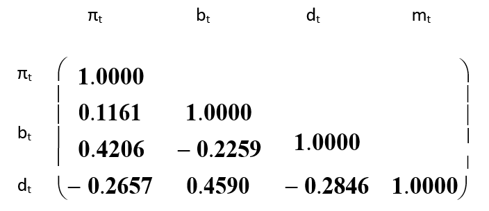
A preliminary step is taken to calculate the correlation matrix for the four variables. The result shows that government external reserve is most correlated with the fiscal deficit to GDP ratio.

The variables are tested for panel unit root and panel stationarity using Im et al. (2003) and Hadri (2000) to determine their degree of integration and level of stationarity. The results of the panel unit root tests are given in Table 3. The result shows that the variables are nonstationary in levels but stationary in first difference, an indication that the variables are integrated of order 1.

The results of the long-run cointegration parameters using the PMGE are given in Table 4. The long-run panel cointegration test results show that these variables, inflation rate, fiscal deficit/surplus to GDP ratio account for most of the gross external reserves in agreement with the results of Catao & Terrones (2003).

Central Bank financing of the fiscal deficit however, did show little influence on the gross external reserves with a low coefficient value of -0.07 with standard error of 0.03. The long-run panel cointegration relation using the PMGE with individual constants is

Equation (24) shows that a 1% increase in government external reserves (mt) induces 0.44% inflation rate (πt). Similarly, a 1% increase in mt will induce a 0.03% increase in the fiscal deficit to GDP ratio, and -0.07% decrease in the Central Bank financing of fiscal deficit. This result compares favorably with Solomon and de Wet (2004) whose simulation study showed that inflation is very responsive to shocks in budget deficit as well as GDP.

In Table 5, the estimation results for the PMGE for the individual countries are reported. The error correction terms have values that are reasonably substantial for most of the countries except Guinea. The estimated value of the error correction term for Guinea is 0.002 which is low compared to the other countries. This may not necessarily be due to inefficiency of the method, but the fact that in the long-run government external reserve is not affected by inflation, fiscal deficit to GDP ratio and Central bank financing of fiscal deficit in Guinea (see Banerjee et al. 1993 for details).

The objective value of the optimum convergence criteria is 0.0452. The objective value for the variables, objective coefficients and their objective value contribution are given in Table 6. Inflation is the highest contributor to the optimum value followed by Central Bank financing of fiscal deposit, while fiscal deficit to GDP ratio is the least.

The conclusion we draw from the paper is that Government external reserves, inflation rate, fiscal deficit/GDP ratio, Central Bank financing of fiscal deficit are correlated with the highest correlation between government external reserves and fiscal deficit and GDP ratio. The result shows that the objective value of 0.0462 is obtained with inflation contributing more to the variation in the government external reserves at variance with the correlation matrix. This may be due to the non-stationarity of the variables in level. Due to the result of linear programming approach, we advise that Central Banks in the countries studied to be cautious in implementing inflation targeting as a way of tackling their economic problems. In conclusion there is a warning by Solomon and De Wet (2004) that governments should note the sensitivity of price levels to fiscal policy.