Numerical Investigation of the Design and Operational Parameters Effects on the Performance of an Axial Micro-Turbine for Hydropower Generation
Abstract:
Axial micro-hydro turbines' performance is sensitive to design and operational parameters. This study investigates the performance of micro-hydro turbines through advanced computational fluid dynamics simulations utilizing ANSYS FLUENT. A three-dimensional, steady-state RANS approach with the SST $k-\omega$ turbulence model was employed to simulate fluid flow interactions in turbines of 3, 4, and 5 blades, multiple rotational speeds of 100 and 1000 RPM, and flow rates. The research uniquely investigates a design that integrates internal flow control features by incorporating secondary guide blades and axial flow straighteners, which effectively reduce vortex formation and energy dissipation. Results show that increasing blade count significantly boosts mechanical power output and hydraulic head across flow conditions. Turbines operating at higher rotational speeds demonstrate markedly enhanced power generation, indicating the importance of mechanical design for durability under elevated stress. Comparative analyses between water and oil as working fluids reveal interesting fluid-dependent performance trends, with oil exhibiting superior energy transfer at higher RPMs. Validation against empirical data confirms the computational procedure's accuracy, with RMSE below 4%. The best performance was observed with the 5-blade turbine, reaching 95%, 92%, and 95% at rotational speeds of 100, 500, and 1000 RPM, respectively, at 60,700 Reynolds number. This configuration consistently outperformed others, demonstrating superior energy conversion. The addition of axial flow straighteners slightly improved efficiency by minimizing turbulence and vortex losses, confirming that structural enhancements combined with high rotational speeds are key to achieving maximum turbine performance.
1. Introduction
Renewable energy technologies now comprise approximately 34% of the global installed power capacity, totaling around 2,179 GW, with hydropower playing a leading role by contributing 1,151 GW, or 18% of the total capacity at an annual growing rate of 1.9% [1], [2]. In light of urgent climate challenges and growing global energy demand, accelerating the transition to a renewable-focused energy mix is essential. Over the next decade, the expansion of large-scale, commercially viable renewable projects, including solar, wind, and hydroelectric power, will be critical in significantly reducing carbon emissions worldwide [3]. Furthermore, supporting low-head hydropower and hydrokinetic energy technologies that harness power from water currents and waves is vital for promoting sustainable industries that utilize untapped renewable resources [4], [5].
Renewable energy systems must emphasize cost-effectiveness, minimal environmental impact, and high power efficiency relative to average annual energy production. Water conveyance systems hold significant untapped renewable energy potential, enabling energy extraction without the need for additional dams or diversions, thereby reducing construction costs and environmental disruption. With appropriate incentives, projects capable of generating at least 1,000 MWh annually could achieve competitive energy prices, estimated between \$0.07 and $0.08 per kWh [6]. In particular, hydrokinetic systems and micro-hydro installations provide reliable and efficient power generation in locations with accessible flowing water, often surpassing conventional energy sources in cost-effectiveness [7]. Supported by organizations such as the European Small Hydropower Association (ESHA) [8], low-head hydropower harnesses energy from water at moderate pressures. HK devices, ideally suited for rivers with adequate flow and reliability, extract kinetic energy from water currents in a manner analogous to how wind turbines capture energy from airflows [9], [10]. These technologies are especially valuable for remote areas, offering low-maintenance, environmentally friendly power generation that helps alleviate the need for large-scale potential energy infrastructure [11], [12].
The environmental impacts on aquatic ecosystems and water quality discussed by Quaranta et al. [13] have encouraged a shift from conventional turbines toward more sustainable and innovative low-head technologies. Emphasizing advantages in low-speed, high-torque scenarios typical of low-head conditions, Akwa et al. [14] differentiate between drag-based Savonius turbines and lift-based Darrieus turbines. Subsequent studies on hybrid turbine models by Saini and Saini [15], as well as hydrokinetic performance analyses of modified turbines by Alam and Iqbal [16], Al-Kayiem et al. [17], and Ma et al. [18], further confirm the superior torque generation of S-rotor turbines, largely attributed to the higher density of water compared to air.
Recent advances in low-head hydropower technologies have garnered increasing research interest. Innovations such as helical and inclined-gate turbines have significantly improved efficiency in ultra-low-head conditions, enabling energy generation at sites previously considered uneconomical [19], [20]. In low-velocity flows, enhanced Savonius rotor designs with aerodynamic improvements have demonstrated notable gains in energy capture efficiency [21]. Additionally, cost-effective small-scale hydrokinetic systems have proven viable for rural electrification, providing reliable and environmentally friendly power to off-grid communities. Micro hydro turbines have been proven to be effective and suitable for small, standalone hybrid renewable energy power systems [22], [23], [24]. Bhayo et al. [25] found that small hydro turbines are a very successful method to be adopted in the Pumped-Hydro-Storage System plants that are utilizing solar PV-battery integrated with hydro turbines for small-scale power generation to support rural communities.
Differing from previous work, the present study employs computational fluid dynamics (CFD) to investigate internal structural modifications within hydraulic turbines, specifically the addition of secondary guide blades and axial flow straighteners (AFS). While the influence of RPM and blade number is well-established, this research uniquely explores how the spatial arrangement of internal AFS, combined with blade configurations, affects flow uniformity, vortex suppression, and mechanical power output. By integrating traditional design parameters with innovative internal flow control features, this study provides a more comprehensive framework for optimizing hydraulic turbines in low-head energy applications.
2. Computational Methodology
ANSYS fluent software has been utilized for the simulation of various design and operational conditions of the micro-hydro turbine. For validation and simulation needs. The CFD modeling of the turbine is naturally complex, considering the turbulent character of the flow around the rotor. Using a 3D steady-state finite volume approach and the incompressible Reynolds Averaged Navier-Stokes (RANS) equations, CFD simulations were run to solve the governing equations and simulate the actual flow field. Pre-processing is critical, as errors in this stage can undermine the entire simulation. These steps of pre-processing lead into the solution phase for simulation of fluid flow, in which the governing equations of flow found frequently in the Navier-Stokes equations are solved numerically using the selected solver. The turbulence model should then be provided along with convergence criteria and settings for the time step, such that the model really represents the behavior of the fluid given the circumstances during the phase of model setup. Post-processing, in which the simulation findings are visualized and examined, marks the concluding stage of this investigation. It covers all the most crucial graphical depictions, including vectors, pressure contours, and streamlines, in order to understand the fluid's behavior within a certain region. In the scope of this study, a fluid domain of the turbine was modeled and efficiently discretized using a structured butterfly mesh. Usually, with a regular connection, the structured mesh permits precision in the capture of the fluid flow around almost essential areas such as turbomachine blades. Figure 1 shows the sequence of the computational procedure.

The computational domain for this study consists of a three-dimensional model of a hydraulic turbine and its surrounding fluid flow region, designed to accurately capture the flow dynamics and performance characteristics. The turbine geometries were developed and analyzed using ANSYS FLUENT 2021 R1, a widely recognized CFD software known for its robustness in simulating turbulent fluid flows in complex geometries. Figure 2 illustrates the overall turbine geometrical model. In all cases of various blade numbers and design configurations, the turbine is kept at a total axial height of 176.5 mm, while the span is kept at 245.5 mm. The blades are fixed on the turbine runner with a height of 65 mm and a thickness of 3 mm. The hub diameter is 122 mm with an axial height of 60 mm.
Previous research has extensively examined the effects of blade count and rotational speed (RPM) on turbine performance, particularly in wind and hydrokinetic systems. Three primary turbines were examined, differentiated by blade count: three blades (3B), four blades (4B), and five blades (5B), as shown in Figure 3. Each turbine model maintained a consistent rotor diameter of 245.5 mm and total length of 176.5 mm to ensure comparability and proper comparisons.
In addition to blade count variations, this study incorporated an investigation of four different designs of internal flow modifications using secondary guide blades and AFS. The four proposed configurations were tested for the 5B turbine, as described in Table 1.
The flow straighteners serve to modify the vortex structures within the flow passage, aiming to reduce energy dissipation caused by turbulent vortices and enhance overall hydraulic efficiency.
All turbine models were subjected to varying operating conditions, including rotational speeds of 100 and 500 RPM, and volumetric flow rates ranging from 0.0049 to 0.0785 m$^2$/s. These conditions enable a comprehensive parametric study of performance across typical real-world operating ranges. Table 2 summarizes the ranges of blade counts, rotational speeds, flow rates, and AFS configurations independently tested to assess their effects on turbine performance.
Configuration | Definition | Numerical Modeling |
|---|---|---|
Bare case | Normal turbine with 5 blades without modification | 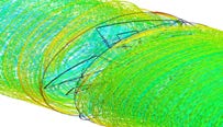 |
Confg (1) | Modified bare 5B turbine by adding axial flow straighteners positioned at the front of the blades | 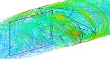 |
Confg (2) | Modified bare 5B turbine by adding axial flow straighteners positioned at the rear of the blades | 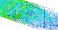 |
Confg (3) | Modified bare 5B turbine by adding axial flow straighteners positioned at the front and the rear of the blades | 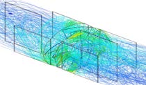 |
Research Variable | Values and Identification |
|---|---|
Liquid flow rate | 0.0049, 0.0196 |
Q $\left(\mathrm{m}^3 / \mathrm{sec}\right)$ | 0.0392, 0.0785 |
Rotational speed (RPM) | 100, 500, 1000 |
Number of blades | 3, 4, 5 |
Configurations with axial flow straighteners | In the front; In the rear; In front and rear |
To simplify the simulation process while maintaining result validity for performance comparison, the following assumptions were adopted:
$\bullet$ The system is assumed to be in steady-state. This assumption is valid as the turbine operates under continuous inflow with no transient fluctuations expected in design evaluation. Unsteady phenomena such as startup or shutdown are outside the scope of this parametric study.
$\bullet$ Physical properties of fluids are considered constant. Since the operating temperature and pressure ranges are narrow and stable, the density and viscosity of water and oil remain effectively unchanged, making this assumption appropriate for accurate performance assessment.
$\bullet$ Thermal effects are excluded as the process of energy conversion is not combined with temperature change or heat transfer. In hydraulic turbines, the influence of temperature on fluid dynamics is minimal under normal operating conditions. Heat transfer has a negligible impact on flow structure or energy conversion, thus not affecting the results of this study.
$\bullet$ Body forces like gravity and energy dissipation due to minor losses are not included. These are insignificant in horizontal flow configurations over short distances and do not affect rotational power output or head significantly.
$\bullet$ The flow is modeled as three-dimensional and turbulent, which reflects the real behavior around the rotor blades. This assumption increases fidelity and does not introduce error, as it closely matches physical conditions.
$\bullet$ Surface roughness of the blades and body is insignificance and surfaces are assumed smooth. In polished or lab-scale prototypes, roughness-induced drag is minor.
Taking into consideration the assumptions mentioned above, the governing conservation equations are as follows:
i. Continuity equation [26], [27]
In which the $x$, $y$, and $z$ components of velocity are denoted by $u$, $v$, and $w$, and provided in Eq. (2), respectively.
ii. Momentum equation
where, $p$ represents the fluid's local pressure, $\mu_f$ is the fluid dynamic viscosity, and $\rho_f$ is the fluid density.
iii. The $k-\omega$ Shear Stress Transport (SST) turbulence model consists of two equations, Eqs. (3) and (4) [26], [27], [28]:
a. The turbulent kinetic energy, $k$:
b. The specific dissipation, $\omega$:
where, $U$ is the mean velocity, $\mu$ and $\mu_t$ are the molecular and turbulent viscosities, respectively, Gk represents the generation of turbulence kinetic energy due to mean velocity gradient, and $S_{\omega}$ and $S_k$ are user-defined source terms. The terms $\alpha, \beta, \sigma_k$, and $\sigma_\alpha$ are the turbulence model constants.
To numerically analyze the flow field surrounding the turbine, turbulence models were incorporated into the Reynolds Averaged Navier-Stokes (RANS) CFD solvers. The most suitable model is the one that yields results in close alignment with experimental findings, thereby demonstrating its accuracy and validity.
In terms of flow boundary conditions, a velocity inlet was selected at the inlet, and a pressure outlet with zero static pressure differential was selected at the outlet (open to atmosphere). The current study's boundary conditions are tabulated in Table 3 and Figure 4. To simulate realistic flow conditions, the computational domain included inlet and outlet flow regions, each extending one meter in length upstream and downstream from the turbine, respectively. These extensions provide sufficient space to minimize boundary effects and allow fully developed flow at the inlet and outlet boundaries.
Domain | Boundary Condition | Value/Setting |
|---|---|---|
Inlet | Velocity inlet | Variable (based on flow rate) |
Outlet | Pressure outlet | 0 Pa (gauge) |
Duct surface | Wall (No slip condition) | Fixed |
Rotating zone | Rotational speed | 100, 500, and 1000 RPM |
Turbulence model | SST $k-\omega$ | Selected for near-wall accuracy |
Fluid | Water and oil | Constant properties |
Mesh | Hybrid mesh, refined near blades | $\mathrm{Y}+<1$ |
Convergence criteria | Residuals | $<1 \times 10^{-5}$ |
Solver | Steady-state, incompressible | 3D RANS, ANSYS FLUENT |
The fluid domain was discretized using a structured butterfly mesh to ensure high mesh quality and accurate resolution near critical regions such as blade surfaces. The mesh was carefully refined to maintain a dimensionless wall distance, Y$^+$, below unity to ensure proper capture of near-wall turbulent effects critical for rotating machinery simulations. In the simulation, the grid that discretizes the flow around the turbine is a circular duct, a three-dimensional unstructured grid with tetrahedral elements. The grid elements near the surface of the turbine were refined in order to capture the important characteristics of the flow in the boundary layer near the surface of the turbine. The height of the first cell was in the order of 0.01 mm, which results in a dimensionless height Y$^+ <$ I. The ANSYS-Meshing module was utilized in grid generation. The meshed domain extends 1 m before and 1 m after the turbine. Figure 5 shows the flow domain around the turbine with the applied boundary conditions.
A mesh independence study was conducted using the 5 Blade turbine. In the independence study, hydraulic efficiency was chosen as the main variable to examine the quality of the mesh. To fulfill this purpose, five different mesh sizes were generated and examined by varying the number of elements. Figure 6 illustrates the variation in hydraulic efficiency with respect to the total number of elements. It can be seen that as the number of elements increases, the hydraulic efficiency varies. In addition, for a grid with a total number of elements of 4,043,265, the solution stabilizes, and no big difference in hydraulic efficiency can be noticed as the number of elements increases beyond this value. Therefore, the number of elements of 4,043,256 was selected for the rest of the simulations.
To ensure the reliability of the turbulence model choice, a brief sensitivity comparison was conducted using a single turbine configuration 4B at 1000 RPM, simulated with both the standard $k-\varepsilon$ and SST $k-\omega$ models. The resulting efficiency difference was less than 2%, confirming that SST $k-\omega$ provides consistent predictions while maintaining higher near-wall resolution. As shown in Figure 6, efficiency values stabilized beyond 4 million mesh elements, indicating that further mesh refinement had a negligible impact on results.
This study used the commercial software package ANSYS FLUENT 2021 R1 to solve governing equations and associated forces. The coupled scheme was utilized to solve the coupling between pressure and velocity. Furthermore, pressure, momentum, turbulent dissipation rate, and turbulent kinetic energy were discretized using the second-order upwind scheme. Table 4 displays the schemes applied in the simulations. Convergence criteria for all simulations were met when the residual error fell below 10$^{-5}$. Figure 7 shows a sample of the variation of residual with the number of iterations. The robustness of the CFD model was evaluated through mesh independence and solver convergence analyses. Additionally, Figure 7 demonstrates that all key residuals (continuity, momentum, turbulence variables) converged to values below 10$^{-5}$, confirming numerical stability and well-resolved flow fields.
Solver sensitivity was tested by comparing results from the SST $k-\omega$ model with the standard $k-\varepsilon$ model for a representative case (4B at 1000 RPM). The variation in predicted efficiency remained within 2%, validating the appropriateness of the selected turbulence model. The SST $k-\omega$ model was selected for this study due to its robustness in predicting flow separation and near-wall behavior, which are essential features in rotating turbomachinery flows. Compared to standard $k-\varepsilon$ and RNG models, the SST $k-\omega$ model offers improved accuracy in adverse pressure gradient regions and better convergence stability for curved blade flows.
Scheme | Type |
|---|---|
Pressure velocity coupling | Coupled |
Pressure | Second order upwind |
Momentum | Second order upwind |
Turbulent kinetic energy | Second order upwind |
Turbulent dissipation rate | Second order upwind |
Turbulence model | $k-\omega$ (SST) |
In fluid dynamics, a key parameter to characterize the fluid and flow is the Reynolds number, Re, which quantifies the proportion of inertial forces to viscous forces in the fluid flow, as in Eq. (5).
where, $\rho$, $U$, and $\mu$ denote the fluid's density, mean velocity, and dynamic viscosity, respectively, while $L$ signifies the characteristic length. When referring to an airfoil, this length typically corresponds to the chord length of the blade.
The overall hydraulic efficiency, $\eta_H$ of the turbine is defined by Eq. (6) as:
The equation relates the mechanical power output of the turbine to the hydraulic energy available in the flow and the dimensionless coefficients defined earlier. All three coefficients, power coefficient, $C_P$, capacity or discharge coefficient, $C_Q$, and head coefficient, $C_H$, are included in the unique performance parameter, the hydraulic efficiency, $\eta_H$. This hydraulic efficiency is the most important parameter in assessing the performance of a turbine, because through this, one can directly determine how much of the energy in the water flow has been converted to useful mechanical power. Eqs. (7)–(9) could predict them.
3. Results and Discussion
Numerical simulation validation was performed by comparing the results on hydraulic efficiency obtained in the current study against the reported results in the literature. Figure 8 shows high similarity in the results trend of the current and Dario et al. [29], in particular, the efficiency results in a 76 mm pipe diameter. The small differences in the values might be due to several reasons: finer mesh resolution used in the present study increased the resolution of the flow, particularly in regions close to the turbine blades. The differences in turbulence modeling or in the specification of boundary conditions may serve as other probable causes of such variance. Despite these differences, the general behavior of the turbine is captured quite well since the efficiency curves are only slightly separated across the flow range.
The general agreement between the two studies certainly gives solid validation to the CFD approach taken herein. These results further reinforce the credibility of the present model, hence positioning it as a reliable tool for further research into performance optimization.
With this in mind, the capability of the current model to capture such subtle variations in fluid dynamics and performance is a clear indication of the potential to accurately simulate advanced turbine configurations for the optimization of energy conversion efficiency.
As shown in Table 5 the efficiency values of the present work closely match the reference data across all tested flow rates. The percentage deviation remains below 4%, with a Root Mean Square Error (RMSE) of approximately 2.46%. This agreement confirms the reliability and accuracy of the numerical model for predicting turbine performance.
Flow Rate ($\mathrm{m}^3 / \mathrm{s}$) | Re | Dario et al. [29] [%] | Present Work [%] | % RMSE |
|---|---|---|---|---|
0.007 | 38,600 | 64.2 | 66.5 | + 3.59% |
0.009 | 49,600 | 63.1 | 64.2 | + 2.74% |
0.011 | 60,700 | 60.4 | 62.1 | + 2.81% |
0.013 | 71,700 | 57.2 | 58.4 | + 2.10% |
0.015 | 82,700 | 54.5 | 55.6 | + 2.02% |
0.0165 | 91,000 | 52.1 | 53.4 | + 2.49% |
Figure 9 shows that the mechanical power production of a turbine at a constant rotational speed of 100 RPM varies with three blades (3B), four blades (4B), and five blades (5B). The produced power is increasing as the flow rate rises. Nevertheless, the pace of rise depends on the number of blades. Also, the turbine with five blades (5B) displays the greatest rise and reaches the maximum power production across almost all flow rates, and reaches the highest power production of 159 W. This information implies that adding more blades to a turbine improves its capacity to transform fluid flow into mechanical energy, hence optimizing turbine designs for particular uses might depend critically on this information.
Figure 10 offers a thorough investigation of how, with each turbine operating at a constant speed of 100 RPM, the number of blades on a turbine affects its hydraulic head losses across varied flow rates represented by Re. As the number of blades increases, the hydraulic losses increase due to the larger contact area between the fluid and the turbine blades. In addition, it is also shown that the losses are increasing with the increase in the flow rate.
Figure 11 provides velocity distribution contours inside the turbine system at a rotational speed of 100 RPM. These simulations show how the blade arrangement affects the flow characteristics and shed light on the fluid dynamics around the turbine blades. Three sections of the figure match distinct blade counts of three blades (3B), in Figure 11a, four blades (4B) in Figure 11b, and five blades (5B) in Figure 11c. As seen by the color scales on the sides of every picture, each segment shows a color-coded velocity contour map wherein the colors reflect varying velocity magnitudes in meters per second.
Comparatively to the other two configurations, the three-blade arrangement exhibits a less homogeneous velocity distribution on its velocity contour. Concentrated directly downstream of the blades, the greatest velocities signal quick flow acceleration over the limited blade surface. Greater energy extraction per blade might follow from this, but it could also produce more turbulence and maybe greater flow separation, therefore reducing the general efficiency.
The velocity profile in the four-blade design seems more homogeneous and smoother around the blade regions when an additional blade is added than in the three-blade configuration. More blades mean less gaps, allowing the fluid to travel unhindered, thereby improving flow control. This regulated flow enhances the kinetic energy transmission to the blades and reduces the possible of turbulence losses. Turbine with five blades (5B) exhibits the most homogeneous flow, with the maximum velocities being efficiently spread across the blades. Unlike the three and four-blade arrangements, which may lower mechanical stresses and preserve flow stability, the flow acceleration is more gradual because less turbulence and more constant blade engagement with the flow imply improved efficiency and maybe better energy conversion capabilities. Increasing the blade count not only influences the energy conversion efficiency but also greatly influences the flow dynamics according to the trend throughout the many configurations. More blades minimize flow separation and so help to stabilize the flow. This stabilization maximizes the transfer of kinetic energy into mechanical power and lets the turbine run more smoothly, therefore extending its mechanical lifetime and durability.
Figure 12 shows the mechanical power output, Pmech, at various flow rates, Q, for three turbine configurations, 3B, 4B, and 5B, under water and oil operational working fluids with 100 RPM turbine operational speed. The flow rates are represented in terms of Reynolds number, ranging from 38,600 to 82,700. Mechanical power increases with flow rate for all cases, consistent with the rise in available kinetic energy. The consistent performance ranking 5B $>$ 4B $>$ 3B in both working fluids further confirms the design robustness. Contrary to expectations based on fluid viscosity, the water-based simulations yield higher power outputs than water at all flow rate ranges. Specifically, at 100 RPM, there is a marked increase in mechanical power output across all blade configurations when using oil. Ultimately, the figure emphasizes that blade count significantly influences turbine performance, and viscous fluids like oil can outperform water under optimized high-speed conditions.
Table 6 presents the hydraulic energy efficiency of turbines with different blade numbers, 3B, 4B, and 5B, operating under varying flow rates, Q, for both water and oil as working fluids. Across all flow rates, the 5-blade (5B) turbine consistently achieves the highest hydraulic efficiency, followed by the 4-blade (4B) and 3-blade (3B) configurations. These results confirm that increasing the number of blades enhances the turbine's ability to convert fluid kinetic energy into useful hydraulic energy.
Re | Turbine Efficiency with Water Flow (%) | Turbine Efficiency with Oil Flow (%) | ||||
|---|---|---|---|---|---|---|
3B | 4B | 5B | 3B | 4B | 5B | |
38,600 | 65 | 70 | 83 | 63 | 69 | 70 |
49,600 | 70 | 75 | 88 | 68 | 72 | 74 |
60,700 | 78 | 83 | 93 | 74 | 77 | 78 |
71,700 | 62 | 66.5 | 74.8 | 59.5 | 62 | 63 |
82,700 | 46 | 50 | 56.5 | 45 | 47 | 48 |
The data also reveal that efficiency generally increases with flow rate up to around 0.03–0.04 m$^3$/s before declining at higher flow rates, indicating an optimal operating window for the turbine designs. At higher flow rates, with Re = 82,700, efficiency drops significantly, likely due to increased turbulence, flow separation, or other losses. This finding is in alignment with the hydraulic losses prediction presented in Figure 10.
However, when comparing the two fluids, water-based turbines consistently exhibit higher efficiencies than their oil-based counterparts at all flow rates and blade counts. This performance difference can be attributed to oil's higher viscosity, which increases flow resistance and reduces energy conversion efficiency. Nonetheless, the relative ranking of blade configurations remains the same in both fluids, demonstrating that blade count is a dominant factor in turbine efficiency regardless of the working fluid.
Figure 13 illustrates the efficiency versus flow rate for various 5-blade turbine configurations, including the bare model and three modified designs incorporating different AFS arrangements. All configurations exhibit consistently high efficiency up to a Reynolds number around 60,000, corresponds to a flow rate of approximately 0.05 m$^3$/s, demonstrating robust performance across moderate flow conditions. Among these, the standard 5B configuration achieves the highest peak efficiency, reaching around 95%. The modified configurations display similar efficiency trends, with higher peak values improved by no more than 5% from the bare case, indicating that the structural changes do not substantially compromise performance. Beyond the 0.05 m$^3$/s flow rate, efficiency declines in all variants, likely due to increased turbulence and flow separation effects at higher velocities, i.e., the turbine is stalled.
The performance comparison of the bare 5B configuration and its three variants, shown in Figure 14 and Figure 15 demonstrates clear differences in mechanical power and head generation across the Reynolds number range investigated.
Results displayed in Figure 14 revealed that the mechanical power produced for all configurations increases sharply at low to moderate Re of 35,000–55,000. Configurations (2) and (4) maintain the highest output power across the full range, with Confg. (2) peaking at approximately 255 W and, as shown in Figure 15, delivering the greatest head of about 1.9 m at Re $\approx$ 85,000. Figure 15 indicates superior hydraulic efficiency under high-flow conditions. Configuration (3) achieves strong mid-range performance, reaching 205 W and 1.6 m head near Re $\approx$ 62,000, but declines at higher Re likely due to increased turbulence losses or flow separation leading to stall phenomena. Configuration (1) offers moderate improvement over the baseline but remains below the top performers, while the baseline consistently records the lowest values, rising gradually to 160 W and 1.3 m head. Overall, the results suggest that the geometric enhancements in Confg. (2) and (4) promote more effective energy capture and pressure conversion across variable flow regimes, whereas Confg. (3) may be best suited for stable, mid-range operating conditions.
Figure 16 quantifies the simulation results in terms of the efficiency of the turbine with 5 blades, 5B, rotating at 100, 500, and 1000 RPM at various flow rates. The flow rates are represented in terms of Reynolds numbers ranging from 35,000 to 85,000. Results indicate that at 500 RPM, the turbine efficiency is high at a low range of Re up to 55000. With higher flow rates, or higher Re, the efficiency of the turbine is slightly higher when the turbine rotates at 100 RPM. However, at all rotational speeds, the decline in efficiency starts after 60,000 Reynolds numbers. The results are compatible with the simulation results reported by Dario et al. [29] for a 5B turbine operates with 2000 RPM.
4. Conclusions
This work simulated an axial flow micro-hydro turbine installed in a liquid pipe flow to generate electrical power. The simulation is performed over a range of 35,000 $<$ Re $<$ 85,000. The results unequivocally demonstrate the significant impact of structural improvements on blade number. Among all tested 3, 4, and 5-blade turbines, the 5-blade arrangement consistently delivered superior performance across a broad range of flow rates, improving average hydraulic efficiency by approximately 24% and mechanical power output by up to 34% compared to the 3-blade configuration. Increasing rotational speed from 100 to 500 and 1000 RPM shows no substantial improved in the turbine efficiency. However, at all tested rotational speeds, the performance decline starts at 60,000 Reynolds number, where the efficiency reduces dramatically after this point for all tested configurations and all tested rotational speeds. With water and oil as options of the working fluid, water consistently produced higher hydraulic efficiencies than oil by 8–12. Internal structural modifications, including optimized AFS positioning, maintained peak efficiencies within 5% of the baseline, 5B, while delivering up to 27% more mechanical power, with installed AFS in the front, in the rear, and in the front and rear, favoring mid-range flows. The study contributes valuable knowledge for retrofitting existing systems or designing next-generation turbines to harness low-grade hydraulic resources more effectively with reduced environmental impact, advancing the global adoption of sustainable renewable energy solutions.
The data used to support the findings of this study are available from the corresponding author upon request.
The authors declare that they have no conflicts of interest.
$D$ | Turbine diameter, m |
$H$ | Hydraulic head, m |
$P_{mech}$ | Mechanical power output, W |
$p$ | Local fluid pressure, Pa |
$Q$ | Volumetric flow rate, m$^3$/s |
$u, v, w$ | Velocity components in x, y, z directions, m/s |
Greek Letters | |
$\mu$ | Dynamic viscosity, Pa·s |
$\rho$ | Fluid density, kg/m$^3$ |
$k$ | Turbulent kinetic energy, m$^2$/s$^2$ |
$\omega$ | Specific dissipation rate, 1/s |
$v$ | Kinematic viscosity, m$^2$/s |
$\mu H$ | Hydraulic efficiency |
Abbreviations | |
$AFS$ | Axial flow straightener |
$CFD$ | Computational fluid dynamics |
$CH$ | Head coefficient |
$CQ$ | Capacity coefficient |
$CP$ | Power coefficient |
$RANS$ | Reynolds Averaged Navier–Stokes |
$Re$ | Reynolds number |
$RPM $ | Revolution per minute |