A DenseNet-Based Deep Learning Framework for Automated Brain Tumor Classification
Abstract:
Brain tumors represent a critical medical condition where early and accurate detection is paramount for effective treatment and improved patient outcomes. Traditional diagnostic methods relying on Magnetic Resonance Imaging (MRI) are often labor-intensive, time-consuming, and susceptible to human error, underscoring the need for more reliable and efficient approaches. In this study, a novel deep learning (DL) framework based on the Densely Connected Convolutional Network (DenseNet) architecture is proposed for the automated classification of brain tumors, aiming to enhance diagnostic precision and streamline medical image analysis. The framework incorporates adaptive filtering for noise reduction, Mask Region-based Convolutional Neural Network (Mask R-CNN) for precise tumor segmentation, and Gray Level Co-occurrence Matrix (GLCM) for robust feature extraction. The DenseNet architecture is employed to classify brain tumors into four categories: gliomas, meningiomas, pituitary tumors, and non-tumor cases. The model is trained and evaluated using the Kaggle MRI dataset, achieving a state-of-the-art classification accuracy of 96.96%. Comparative analyses demonstrate that the proposed framework outperforms traditional methods, including Back Propagation (BP), U-Net, and Recurrent Convolutional Neural Network (RCNN), in terms of sensitivity, specificity, and precision. The experimental results highlight the potential of integrating advanced DL techniques with medical image processing to significantly improve diagnostic accuracy and efficiency. This study not only provides a robust and reliable solution for brain tumor detection but also underscores the transformative impact of DL in medical imaging, offering radiologists a powerful tool for faster and more accurate diagnosis.
1. Introduction
Brain tumors are potentially fatal illnesses brought on by the brain's aberrant cells growing out of control. The location and category of these tumors have a major influence on neurological function, causing a variety of symptoms, including headaches, seizures, and cognitive impairments (Saleh et al., 2020). Early accurate diagnostics are the basis for effective therapies and increasing survival rates. Radiologists manually assess Magnetic Resonance Imaging (MRI) as part of standard diagnostic procedures. This is a laborious process that is subject to human interpretation errors. Medical imaging has been transformed by advances in deep learning (DL), especially Convolutional Neural Networks (CNNs), which allow for accurate and automated processing of brain MRI data.
DL stands for disciplines of Artificial Intelligence (AI) that learn characteristics and spot patterns in data using neural networks. Images and other grid-like data are processed using CNNs, which are specialized DL architectures (Alqudah et al., 2020; Sharma et al., 2020). Starting with basic patterns like edges and working their way up to more intricate structures like tumor borders in Figure 1, they employ convolutional layers to extract characteristics in a hierarchical manner. Because CNNs can analyze huge volumes of image data fast and lessen the need for manual feature extraction, they have shown remarkable efficacy in medical imaging for tumor identification and classification (Rasool et al., 2022). CNNs can recognize patterns that distinguish between healthy and diseased tissues, including pituitary tumors, meningiomas, and gliomas, by training on labeled datasets.

Recurrent Convolutional Neural Networks (RCNNs) expand upon the advantages of CNNs by adding recurrent layers, which capture contextual and spatial connections amongst features (Khan et al., 2022). RCNNs improve CNNs' proficiencies in spatial feature extractions by considering connections between various image components. Contextual information (Lakshmi et al., 2023) enables more accurate classifications of brain tumor identifications, which makes RCNNs useful for identifying different tumors or evaluating irregular borders. Convolutional and recurrent layer integration is useful in high-precision medical imaging tasks.
The use of DL in brain tumor detection has produced notable advantages. CNN/RCNN-powered automated systems analyze MRI more quickly and reliably, relieving radiologists from workloads and increasing the diagnostic precision (Gao et al., 2022; Kokila et al., 2021) as they spot even minute patterns and irregularities that human evaluations miss. However, because they assume spherical clusters, classic segmentation techniques like k-means clustering sometimes require assistance with uneven tumor borders. This restriction may lower the accuracy of other processes, such as feature extraction and classification.
A Densely Connected Convolutional Network (DenseNet) architecture for automated brain tumor identification was proposed in this research. The technique starts with segmentation using Mask Region-based Convolutional Neural Network (Mask R-CNN) and pre-processing using adaptive filters to eliminate noise from MRI. Mask R-CNN overcomes the drawbacks of conventional methods by enabling accurate, pixel-level segmentation (Choudhury et al., 2020; Latif et al., 2021). Gray Level Co-occurrence Matrix (GLCM), which records texture-related characteristics, extracts features and tumor types are classified into gliomas, meningiomas, pituitary tumors, or non-tumorous categories using the DenseNet architecture, which is known for effective feature reuse through densely linked layers. The suggested methodology combines sophisticated segmentation and classification algorithms in order to overcome the shortcomings of current systems. While DenseNet guarantees effective processing of complicated feature representations, it improves accuracy by managing uneven tumor borders. This method is a viable way to incorporate DL into clinical operations as it increases diagnostic precision and provides scalability and dependability.
2. Literature Review
Jia & Chen (2020) suggested brain tumor segmentation using Fully Automatic Heterogeneous Segmentation with Support Vector Machines (FAHS-SVM) where automated methods based on anatomical, morphological, and relaxometry parameters scan the cerebral venous system in MRI scans. High degrees of consistency between structures and surrounding brain tissues are indicative of the segmentation. One or more layers of hidden nodes in Extreme Learning Machine (ELM) learning analyze data and learn using probabilistic neural networks in classifications. The work’s numerical findings precisely identified both normal and diseased brain tissues in MRI, demonstrating the efficacy of the technique. Chellakh et al. (2023) introduced deep rule-based (DRB) classifiers for brain tumor classification in MRI, where features extracted using AlexNet, Visual Geometry Group (VGG)-16, Residual Network (ResNet)-50, and ResNet-18 were compared and evaluated for their performance. For classification, a DRB classifier was employed. The first database uses two Kaggle website datasets that are available to the public: tumor and no tumor. Meningiomas, gliomas, and pituitary tumors are all included in this multiclass database. Notable results were obtained from experimental data. A comparative analysis with other state-of-the-art distance methodologies and traditional methods demonstrated the suggested strategy’s efficacy in classifying brain tumors on MRI samples.
Malla et al. (2023) recommended Deep Convolutional Neural Networks (DCNNs) based on transfer learning for the categorization of brain tumors into pituitary, glioma, and meningioma. Visual Geometry Group Network (VGGNet) is a pre-trained DCNN architecture that transfers learning parameters to target datasets after extensive training on large datasets. It also improves the performance by freezing and fine-tuning the neural network's layers. To overcome problems with data overfitting and vanishing gradients, the proposed solution includes Global Average Pooling (GAP) layers at outputs. The suggested architecture was evaluated and compared to other DL-based algorithms for classifying brain tumors on Figshare datasets. Haq et al. (2022) used enhanced CNNs to categorize brain tumors from brain MRI data. The usage of data augmentation and the transfer learning approach enhanced models’ classification, resulting in high prediction accuracy when compared to the baseline models. The suggested method could be used to detect brain tumors in healthcare systems based on the Internet of Things (IoT). Bhanothu et al. (2020) provided Faster R-CNNs by employing the Region Proposal Network (RPN) to locate and localize tumors. The three most frequent forms of brain cancers identified in MRI were pituitary tumors, gliomas, and meningiomas. The VGG-16 architecture served as foundational layers for classifiers and regional suggestions in the suggested method. The classification of the algorithm demonstrated that it had an average level of precision in detecting pituitary tumors, meningiomas, and gliomas.
Ullah et al. (2023) presented TumorDetNet, an integrated end-to-end DL network for classifying and detecting brain tumors. 48 convolution layers with leaky ReLU and ReLU activations were used to produce most unique deep feature maps. Dropout layers and average pooling found distinct patterns and reduced data overfitting. Brain tumors were identified and categorized using softmax and fully connected layers. Their results on six popular Kaggle brain tumor MRI datasets successfully identified meningioma, pituitary, and glioma tumors, classified benign and malignant brain tumors, and detected brain malignancies, demonstrating the accuracy of classifying brain tumors. Saxena & Singh (2024) suggested two CNN designs (DenseNet169 and DenseNet201) for brain tumor identification. The models of DenseNet169 and DenseNet201 were trained on large MRI datasets of brain tumors of all sizes and types. The wide range of links between these models facilitates feature reuse and data interchange, which boosts tumor localization accuracy and performance. The separate testing dataset evaluates trained models, and performance metrics like accuracy and loss were examined where results demonstrated the efficacy of both models. In terms of test accuracy, train accuracy, train loss, and test loss, DenseNet201 performed better than DenseNet169, ResNet-50, and VGG19.
Fakouri et al. (2024) classified brain cancers in MRI using ResNet architectures. The MRI quality of 159 individuals from cancer image archives was enhanced by Gaussian and median filters. In addition, image edges were identified by edge detection operators. The training process involved two stages: the network was initially trained on the original images, followed by the incorporation of preprocessed images enhanced with Gaussian and median filters. This two-stage approach was demonstrated to improve the performance of the DL network, as evidenced by the experimental results. Stephe et al. (2024) suggested automated tumor detection and classification in MRI using the Osprey Optimization Algorithm (OOA) with DL (BTDC-OOADL). The Wiener filtering (WF) model was used in the BTDC-OOADL technique to remove noise. The BTDC-OOADL method uses the MobileNetV2 technique to extract features. OOA was used for the MobileNetv2 model's optimal hyperparameter selection. The Graph Convolutional Network (GCN) model can recognize and classify brain tumors. The experimental results can be evaluated using benchmark data. The simulation results suggest that the BTDC-OOADL system improves with new methods.
Veeramuthu et al. (2022) introduced combined feature and image-based classifiers (CFIC) that use features and images to categorize brain tumors. Actual image feature-based classifiers (AIFC), segmented image feature-based classifiers (SIFC), exacted features and segmented image feature-based classifiers (ASIFC), actual image-based classifiers (AIC), segmented image-based classifiers (SIC), and actual and segmented image-based classifiers (ASIC) with CFIC were all part of the architecture for image classification based on various deep neural networks and DCNNs. The proposed classifiers were trained and tested using the brain tumor detection 2020 dataset from Kaggle. In terms of the acquired accuracy, specificity, and sensitivity values, CFIC performed better than the other classifiers. The proposed CFIC method performs better than the existing classification methods.
3. Proposed Methodology
This work proposes a unique DL-based classification technique, DenseNet, for handling issues highlighted in this study, aiming to categorize brain tumors in order to increase human longevity and lower the death rate. The suggested low-complexity technique classifies brain malignancies accurately compared with other methods. Figure 2 shows the four phases of the recommended technique. An adaptive filtering technique was used for pre-processing in the first phase, and the Mask R-CNN was used for segmentation in the second phase. In the third phase, feature extractions were carried out using GLCM. DenseNet was used in the fourth phase for classification.
Pre-processing is a crucial step for identifying and classifying brain tumors from MRI. The adaptive filter plays a central role in enhancing image quality by removing noise while preserving essential features like edges, which are critical for accurate tumor detection and segmentation (Irmak, 2021). Pre-processing minimizes noise and distortion in images to enhance segmentation precision. Techniques like median filtering preserve edges while smoothing, and adaptive filtering adjusts dynamically to image variations, ensuring cleaner and more accurate images ready for segmentation.
The adaptive filter adjusts dynamically to the local characteristics of the image. It calculates the denoised pixel value $\hat{I}(x, y)$ using the local mean ($\hat{\mu}_L$) and variance ($\hat{\sigma}_y^2$) within a defined window, along with the global noise variance ($\sigma_y^2$) as per Eq. (1).
The filter performs as follows:
Noise-free regions: If $\sigma_y^2=0$, indicating no noise, the pixel remains unchanged, which can be expressed by Eq. (2).
Edge preservation: In areas with high local variance of $\hat{\sigma}_y^2>\sigma_y^2$, the filter retains details such as edges, crucial for distinguishing tumor boundaries.
Uniform regions: When $\hat{\sigma}_y^2 \approx \sigma_y^2$, the pixel value smoothens towards local means and it can be expressed by Eq. (3).
Adaptive filters optimize the balance between noise reduction and feature preservation, where edges and other characteristics are preserved while smoothing uniform areas by examining local variations. This improves identification and classification of malignancies such as gliomas, meningiomas, and pituitary tumors and guarantees high-quality inputs for segmentation and classification. The dependability of DL models in medical imaging is enhanced by the usage of adaptive filters in MRI pre-processing.
Mask R-CNN, a DL model designed for instance segmentation, is ideal for brain tumor segmentation in MRI (Hussain & Khunteta, 2020). It extends Faster R-CNN by adding a pixel-level segmentation branch to detect and segment tumors accurately. The process involves feature extraction, region proposal, bounding box refinement, and mask generation.
The input MRI is passed through a backbone network like ResNet or ResNeXt, which extracts a feature map. This feature map highlights essential patterns in the image, such as edges and textures, critical for detecting tumors. The feature map serves as the basis for region proposal and segmentation.
RPN identifies Regions of Interest (ROIs)—areas in the feature map likely to contain a tumor. It generates anchor boxes of various sizes and aspect ratios and assigns a score to each, indicating the probability of containing a tumor, as shown in Figure 3. The RPN loss function optimizes both classification and localization represented in Eq. (4).
where, $L_{C l s}$ is the classification loss for distinguishing tumor and non-tumor regions, and $L_{r e g}$ is the regression loss for refining the anchor box coordinates.
Detected ROIs are mapped back to the feature map using ROI Align, which resolves spatial misalignment issues caused by ROI pooling in previous methods (Shabu & Jayakumar, 2020). This alignment is achieved via bilinear interpolation, ensuring pixel-level precision can be expressed by Eq. (5).
where, $F(i, j)$ represents feature map values, and $w_{i, j}$ are the interpolation weights.
Each aligned ROI undergoes classification to determine if it contains a tumor and what type. Simultaneously, the bounding box is refined to better localize the tumor.
where, $L_{C l s}$ classifies the ROI (e.g., gliomas, meningiomas, or non-tumor) and $L_{r e g}$ adjusts the size and location of the bounding box.
For each ROI classified as a tumor, a segmentation mask is generated using a convolutional mask branch. This branch outputs a binary mask that segments the tumor from the surrounding tissue. The mask prediction is optimized using the binary cross-entropy loss, as expressed by Eq. (7).
where, $y_i$ is the ground truth mask for pixel $i$; $\hat{y}_i$ is the predicted mask probability for pixel $i$; and $N$ is total number of pixels in the ROI.
MRI is input into the network and passed through the backbone to generate feature maps. RPN identifies ROIs, which are refined and aligned using ROI Align. Finally, the mask prediction branch outputs pixel-level segmentation masks for the detected tumor regions, ensuring precise and accurate delineation of tumor boundaries (Kordemir et al., 2024). After the model produces the final output, such as building boxes around detected tumors, classification labels, categorizing tumors, or marking them as non-tumor and pixel-level segmentation masks, it accurately delineates tumor boundaries, as shown in Figure 3.
The total loss function combines contributions from RPN, bounding box refinement, and mask prediction.
This ensures that all components—region detection, classification, and segmentation—are optimized for precise tumor segmentation. By integrating these components, Mask R-CNN excels at segmenting brain tumors in MRI scans. It is capable of handling irregular tumor boundaries, producing pixel-level masks, and maintaining high accuracy, thereby making it indispensable in medical imaging and diagnostics.
Texture analysis helps machine learning (ML) algorithms and visual perception distinguish between healthy and sick tissues. Additionally, it highlights the distinction between healthy tissues and cancerous growth that could otherwise go unnoticed. Accuracy can be improved by selecting significant statistical criteria for early diagnosis (Nasrudin, 2024). GLCM may be used to obtain second-order statistical texture information. One may determine the frequency with which pixels with specified values and a certain spatial relationship appear in an image by first constructing a GLCM and then utilizing it to extract statistical metrics.
GLCM counts frequencies for statistical evaluations of image textures. It is made up of pixel pairs with identical values and relative positions. GLCM functions can extract statistical information that can be used to describe the texture of an image by determining the frequency of pixel pairings with a specific weight and spatial relationship. In GLCM, a two-dimensional histogram, each pair of p and q denotes the frequency at which they occur. It makes use of the grayscales of p and q, the distance of S = 1, the angle (with 0, 45, 90, and 135 degrees representing horizontal, positive diagonal, vertical, and negative diagonal, respectively), and the understanding that, at a specific distance S and orientation, a pixel of intensity p looks close to a pixel of intensity q. Figure 4 shows the GLCM feature extraction for generation.
In this study, five distinct statistical features are extracted from GLCM after its calculation. These features are essential for capturing various texture properties of the image, as described below:
Contrast: Identifies GLCM's local deviations.
Homogeneity: Determines proximities of GLCM element distributions to its diagonals.
Dissimilarity: Measures the intensity range of grayscale.
Energy: Reflects pixel uniformity.
Correlation: Determines the average degree of connectivity between each pixel in the image and its neighbors.
where, i and j denote the co-occurrence matrix indices; P(i, j) denotes the elements of the co-occurrence matrix at position (i, j); µx and µy denote the averages of row and column weights in the matrix; and $\sigma x$ and $\sigma y$ represent the standard deviations of row and column weights in the matrix.
GLCM’s ability to extract meaningful texture-based features makes it an integral part of the brain tumor classification workflow (Özkaraca et al., 2023). By combining these features with advanced classification models, the approach achieves high accuracy and reliability.
DenseNet is a cutting-edge DL model, known for its densely connected layers, making it efficient and powerful in classifying gliomas, meningiomas, pituitary tumors, and non-tumor cases from MRI (Sabila & Tjahyaningtyas, 2024) and by leveraging its unique feature-propagation mechanisms.
DenseNet connects each layer directly to all subsequent layers in the network. Unlike traditional CNNs, where each layer feeds into the next sequentially, DenseNet enables all layers to share information, optimizing feature extraction and gradient flow.
where, $x_1$ represents the output of layer $l$; $H_l$ represents the composite functions, i.e., Batch Normalization (BN), ReLU activation, and convolution); and $\left[x_0, x_1, \ldots . ., x_{l-1}\right]$ is the concatenation of all preceding layer outputs. This connectivity reduces redundancy, ensures efficient parameter usage, and improves gradient flow, leading to better classification performance.
Dense blocks: These are groups of layers where outputs are concatenated instead of being added, allowing all layers to share features. Each dense block uses the transformation.
This architecture ensures that the model reuses learned features, capturing tumor-specific details like size, shape, and texture.
Growth rate ($k$): Defines feature maps added to layers where smaller $k$ ensures efficient usage of parameters, while a larger $k$ captures more complex tumor features.
Transition layers: Located between dense blocks, these layers compress the network by reducing spatial dimensions and feature maps using a 1 × 1 convolution followed by pooling.
After the dense blocks, GAP layers convert feature maps into compact vectors, which are then input to fully connected layers, with the final output class probabilities being determined through a softmax activation function.
where, $p_i$ is the probability of the input belonging to class $i$; $z_i$ represents the logit score for class $i$; and $C$ indicates a number of classes (gliomas, meningiomas, pituitary tumors, and non-tumors).
As shown in Figure 5, the dense block in a densely linked convolutional network must have the same feature map size before concatenation can be performed between blocks (Wakili et al., 2022). While keeping the feature map size constant, it should be noted that down-sampling is a crucial element in a CNN, which can be accomplished by conducting convolution and pooling outside of dense blocks. The layers responsible for convolution and pooling are known as transition layers. In DenseNet designs, transition layers encompass batch-norm layers, 1 × 1 convolutions, and 2 × 2 average pooling, where 1 × 1 convolutions down-sample input features and produce outputs.
The model is optimized using the categorical cross-entropy loss function.
where, $N$ is the sample count, $C$ is the number of classes, $y_{i, j}$ represents the ground truth for sample $i$ and class $j$, and $\hat{y}_{i , j}$ denotes the predicted probability for sample $i$ and class $j$.
The training involves stochastic gradient descent (SGD) with learning rate scheduling, ensuring effective convergence. Data augmentation (e.g., rotation, flipping, and scaling) is employed to make the model robust to variations in MRI scans.
DenseNet's efficient architecture ensures that even with limited MRI data, it extracts tumor-specific features with high precision, achieving robust and reliable classification. This is crucial for aiding medical professionals in diagnosing and planning treatments for brain tumor patients.
4. Results and Discussion
This proposed model used the Kaggle dataset to test the suggested methods. The two categories of this dataset were testing and training. Glioma tumor, meningioma tumor, pituitary tumor, and non-tumor photos were all included in each training and testing set. The testing set consisted of 394 images, while the training set comprised 2,870 images. Data preprocessing techniques like brain stripping enhanced descriptions of data. Glioma, meningioma, non-tumor, and pituitary tumors were the categories for performance evaluation. Examples of several tumor categories in various locations are depicted in Figure 6 (Bhuvaji, 2020).
Dataset: https://www.kaggle.com/sartajbhuvaji/brain-tumor-classification-mri
The suggested approach was implemented in Python, a high-level ML programming language using Keras, and TensorFlow to create neural networks. This is advantageous for both Central Processing Unit (CPU) and Graphics Processing Unit (GPU) processing. The hyper-parameters were adjusted using a network search, with the parameters selected based on the model’s performance on the validation set. Variables like energy and testing rate changed as the test was being conducted. The learning rate was first set at 0.003 and then gradually decreased to 0.3 × 10⁻⁵; the energy was first set at 0.5 and then increased to 0.9.
In terms of evaluation parameters, five performance metrics—specificity, sensitivity, accuracy, precision, and F1-score—were used to assess the effectiveness of the suggested DenseNet-based framework for classifying brain tumors. These metrics together offer a thorough evaluation of the model's capacity to distinguish between tumor and non-tumor instances while correcting classification discrepancies. False positives, false negatives, true positives, and true negatives were the primary data used to create the metrics.
Input Image | 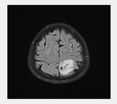 |
Processed Image | 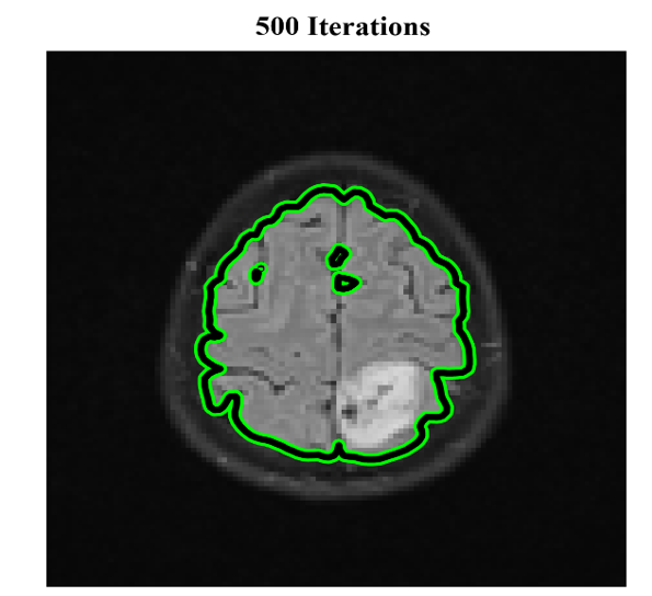 |
Segmentation | 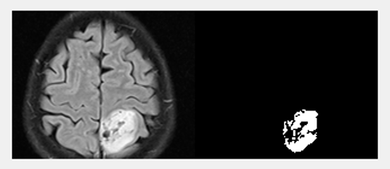 |
Classification | 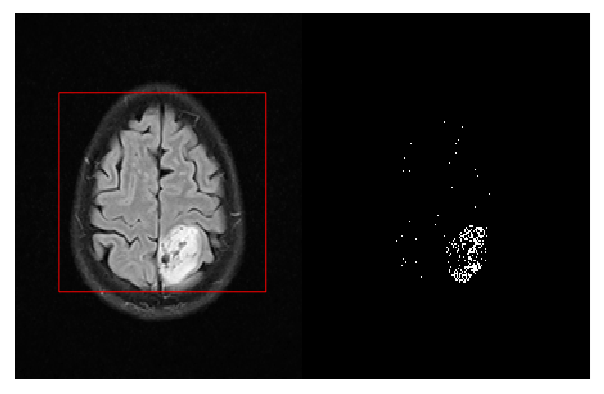 |
Parameter | BP | U-Net | RCNN | Proposed DenseNet |
Sensitivity | 97.87 | 97.51 | 98.42 | 98.84 |
Specificity | 75.47 | 80.39 | 89.28 | 93.43 |
Accuracy | 88.83 | 90.86 | 95.17 | 96.96 |
Precision | 85.50 | 88.68 | 94.34 | 96.59 |
F1-score | 91.22 | 92.80 | 96.34 | 97.70 |
The experimental results were derived from the MATLAB implementation, which processes MRI through segmentation, feature extraction, and classification. The processed results for each step are systematically illustrated in Table 1, which highlights the incremental improvements achieved during the workflow. The overall evaluation metrics and their corresponding formulas, as detailed in Table 2, elucidate how each metric reflects the model's performance.
Sensitivity (recall): The ratio of the number of true positives and false negatives, which can be expressed by Eq. (19).
Specificity: The ratio of true negatives to different false positives and true negatives, which can be used to assess the specificity of brain tumor detection.
Accuracy: The ratio of the precise values found in the population.
Precision: The ratio of true positives to the sum of true positives and false positives.
F1-score: The F1-score value can be calculated by Eq. (23).
Figure 7 illustrates the sensitivity performance of four classification methods: Back Propagation (BP), U-Net, RCNN, and the proposed DenseNet. Among these, the proposed DenseNet achieves the highest sensitivity, approximately 98.84%, demonstrating its superior capability in correctly identifying true positive cases. The RCNN method follows closely with a sensitivity of 98.42%, indicating robust detection accuracy. BP and U-Net methods exhibit slightly lower sensitivity levels of 97.87% and 97.51%, respectively. These results highlight the proposed DenseNet’s effectiveness in ensuring minimal false negatives, which is critical for accurate tumor detection.
Figure 8 compares the specificity of the same four methods. The suggested DenseNet achieves the highest specificity of 93.43%, outperforming others and indicating superior ability to correctly identify true negative cases (non-tumor instances) while minimizing false positives. RCNN comes second with an 89.28% specificity, demonstrating the potent ability to lower false alarms. The specificities of U-Net and BP are lower, at 80.39% and 75.47%, respectively. The outcomes highlight the reliability of the suggested DenseNet in differentiating non-tumorous patients while lowering diagnostic mistakes.
Figure 9 demonstrates accurate categorization with the greatest accuracy of 96.96% achieved by the proposed DenseNet, demonstrating its overall superior performance in accurately categorizing tumor instances. RCNN comes second with an accuracy of 95.17%. BP has the lowest accuracy of 88.83%, while U-Net attains an accuracy of 90.86%. These outcomes highlight the sophisticated design and effective feature extraction techniques of the suggested DenseNet, which produce incredibly accurate classification.
Figure 10 presents the precision performance of the four methods, highlighting their abilities to minimize false positives. The best precision of 96.59% is attained by the proposed DenseNet, demonstrating its capacity to accurately detect real positive cases with little misclassification. 94.34% accuracy is attained by RCNN, 88.68% by U-Net, and 85.50% by BP. The outcomes confirm that the suggested DenseNet performs better at correctly detecting tumor instances while lowering the possibility of false alarms.
F1-score balances precision and recall (sensitivity) values. As shown in Figure 11, the proposed DenseNet's exceptional balance between sensitivity and accuracy is demonstrated by its greatest F1-score of 97.70%. With an F1-score of 96.34%, RCNN comes in second, demonstrating dependable performance. BP has the lowest F1-score at 91.22%, while U-Net has an F1-score at 92.80%. These outcomes demonstrate that the suggested DenseNet is resilient in reaching a high degree of classification accuracy while preserving sensitivity and precision.
5. Conclusions
The proposed DenseNet-based framework for brain tumor classification combines adaptive filtering for noise reduction (with an impressive accuracy of 96.96%), Mask R-CNN for accurate tumor segmentation, and DenseNet for effective feature extraction and classification. This method improves the identification of tumor categories, such as gliomas, meningiomas, pituitary tumors, and non-tumors, and tackles difficulties in irregular tumor border segmentation. Even though the method performs better than existing models like BP, U-Net, and RCNN, its computational complexity and training needs still allow for improvement. To further increase accuracy and therapeutic application, future research should concentrate on maximizing the model's computing efficiency and integrating multimodal data, such as genetic and clinical information.
The data used to support the research findings are available from the corresponding author upon request.
The authors declare no conflict of interest.