Climate–Industry Interplay in Coastal Air Quality: A Comparative Sentinel-5P Study of the North Atlantic and Gulf of Mexico
Abstract:
Coastlines host dense human activity that concentrates combustion and elevates carbon monoxide (CO) and nitrogen dioxide (NO₂) burdens. Yet complex coastal meteorology often limits ground monitoring. We address this gap with a multi-year, dual-pollutant, jurisdiction-scale analysis using a transparent Sentinel-5P column-burden workflow. We employ the workflow on Canada’s Nova Scotia (NS), a cool and relatively stable North Atlantic coast, and the US state of Louisiana (LA), a warm-humid Gulf coast with one of the densest refining hubs, providing two contrasting coastal domains. We analyse 2019-2024 tropospheric column CO and NO₂, apply uniform quality-assured screening, generate time series composites at native resolution, classify spatial fields with Jenks Natural Breaks, and examine temporal trends. Columns are compared with inventories and ground networks as consistency checks. Six-year means highlight persistent contrasts: NS’s column CO is slightly higher than LA’s (0.0338 vs. 0.0321 mol m⁻²), and NS’s NO₂ is ≈ 2.5× LA’s (6.09×10⁻⁵ vs. 2.39×10⁻⁵ mol m⁻²). In NS, NO₂ peaks in summer, while CO reaches its highest seasonal mean in spring; in LA, NO₂ peaks in winter and CO peaks in spring. Recurring hotspots appear over Halifax-Dartmouth and North Sydney, and along the Baton Rouge-New Orleans corridor and northern parishes. These patterns may reflect a combined influence of coastal setting, seasonal atmospheric structure, and local activity, although direct meteorological attribution was not performed. By integrating satellite archives with ground networks, the study provides a reproducible, auditable approach that translates seasonal column dynamics into jurisdiction-ready evidence for evaluation calendars and corridor-focused siting, improving the timing and targeting of coastal air-quality management, and supporting United Nations Sustainable Development Goals (SDGs) 3 and 11.1. Introduction
Water covers about 71% of the planet. Coastal areas, while relatively narrow bands of land, host roughly 40% of the world’s population (Lin & Yu, 2018) and anchor major ports, refineries, and trade corridors, corridors that concentrate combustion sources and elevate carbon monoxide (CO) and nitrogen dioxide (NO₂) burdens (Athul et al., 2025). Studying these pollutants in coastal regions is globally significant in helping meet the Paris Agreement’s Nationally Determined Contributions (Dencer-Brown et al., 2022). Along with complying with the International Maritime Organization International Convention for the Prevention of Pollution from Ships Annex VI controls (Singh, 2023), on ship emissions (e.g., the IMO 2020 sulphur cap (Yoshioka et al., 2024) and Nitrogen Oxides Tier III standards in Emission Control Areas (Gren et al., 2021)). As well, for aligning with the World Health Organization 2021 Air Quality Guidelines (World Health Organization, 2021), and United Nations Sustainable Development Goals (SDGs) targets 3 and 11 (Yue et al., 2024), which all depend on accurate assessment of combustion-driven burdens along shipping corridors, ports, and coastal urban networks. Similar challenges in sustainable transport emissions, such as aviation routes linking coastal regions, underscore the value of collaborative public-private policies and consistent offset standards, which motivate broader participation in pollution reduction actions (Tandamrong et al., 2025). Ground-based monitors provide high-precision point measurements necessary for regulatory needs, such as exposure assessment (Ukhov et al., 2020). However, they lack the spatial coverage required to capture the spatial heterogeneity of pollution, especially in coastal areas where maritime-continental interactions, boundary-layer processes, and meteorological complexities help to drive unique dispersion behaviours (Zhang et al., 2022). Satellite-derived column concentrations, despite providing integrated atmospheric column values rather than at-surface emitted concentrations, have recently been shown to fill a important knowledge gap for analysing pollution dynamics across various spatial contexts (Fioletov et al., 2022; Kenis & Loopmans, 2022). Thus, Sentinel-5P, which offers high spatial resolution (~3.5 × 5.5 km²) (Fioletov et al., 2022; Ukhov et al., 2020) is required to reveal spatial CO and NO₂ patterns, from urban belts around the coastline to regions away from shore, that ground monitors are entirely unable to capture.
Despite important advances, most satellite or inventory-based studies remain short-window (months, 1-2 years) (Johansson et al., 2017; Sofiev et al., 2018), single-pollutant such as CO or NO₂, not both (Douros et al., 2023; Yilmaz et al., 2023), and city- or site-centric rather than jurisdiction-scale (Liu et al., 2024; Kurchaba et al., 2022). Furthermore, many analyses apply heterogeneous quality assurance screens or mix Level-2/Level-3 products without documenting thresholds, impeding comparability e.g., (Wu et al., 2019) and (Pinto et al., 2020); others omit area-/observation-weighting and admin-unit aggregation (Goren et al., 2023; Li & Managi, 2022), and few offer/release code, parameter files, and versioned data needed for full reproducibility (Kedron & Frazier, 2022; Maxwell et al., 2022). Moreover, most coastal applications emphasize statistical associations rather than process attribution, giving limited treatment to marine boundary layers, nocturnal/thermal inversions, sea-/lake-breeze recirculation, synoptic advection, and storm passages that reshape column burdens e.g., (Shetty et al., 2024) and (Douros et al., 2023). Few studies pair columns with boundary-layer height, wind/thermal structure, or trajectory diagnostics to interpret variability mechanistically (Horner et al., 2024; Krol et al., 2024). Many studies implicitly equate satellite columns (mol m⁻²) with surface concentrations (ppm/µg m⁻³) or bottom-up emissions (tonnes), applying direct regressions that ignore units, vertical representativeness, spatial support, and averaging kernels, thereby overstating agreement e.g., (Boersma et al., 2016) and (Dressel et al., 2022). A more appropriate use is direction/magnitude concordance as a consistency check, not equivalence (Cooper et al., 2022; Judd et al., 2019). Accordingly, the unresolved gap is a multi-year, dual-pollutant, jurisdiction-scale assessment for coastal regions that (i) uses high-resolution Sentinel-5P column burdens within a transparent, reproducible pipeline and (ii) interprets patterns through coastal process lenses while treating inventories/ground data as consistency checks rather than surrogates (Athul et al., 2025). Recent bibliometric analyses of coastal management in the blue economy context further highlight fragmented knowledge and persistent gaps in policy integration, technological monitoring innovation, and equitable mechanisms-underscoring the timeliness of jurisdiction-scale, evidence-based approaches (Kismartini et al., 2026).
To address the gap identified above, we analyse 2019-2024 Sentinel-5P column burdens of CO and NO₂ across two climatically and geographically distinct coastal jurisdictions: Nova Scotia (NS) and Louisiana (LA). We employ a transparent, repeatable workflow that treats satellite-retrieved columns explicitly as column concentration diagnostics and interprets observed patterns in relation to possible coastal-process influences, including boundary-layer mixing, maritime ventilation, and seasonal atmospheric stability. Building on this foundation, our study extends Sentinel-5P analysis through a coastal, jurisdiction-scale framework built for governance: its novelty lies in a fixed, auditable, dual-pollutant pipeline that uses seasonal column dynamics to inform evaluation calendars, corridor-specific monitoring priorities, and future equity-aware network planning where appropriate demographic or vulnerability data are available. This study advances beyond descriptive mapping in three ways. First, we implement a fixed dual-pollutant pipeline that enforces identical masking, compositing, and area-weighted aggregation across years and jurisdictions, enabling comparability without case-specific tuning. Second, we summarise multi-year column archives using operationally relevant indicators, including seasonal amplitude, peak timing, hotspot persistence, and anomaly years, so results can inform evaluation calendars and corridor priorities rather than static annual averages. Third, we use the NS-LA contrast as a structured comparative case to examine whether seasonal phasing, interannual co-variability, and hotspot persistence differ across two coastal settings with distinct climatic and industrial characteristics. Our objectives are to: (1) characterise jurisdiction-scale spatiotemporal variability in 2019-2024 CO and NO₂ columns, including disruption and recovery features evident in the 2020-2021 period; (2) interrogate seasonal and interannual behaviour via a systematic comparison of maritime-influenced (NS) versus humid-subtropical (LA) regimes; and (3) assess satellite-surface consistency as a representativeness diagnostic to inform hybrid monitoring protocols. We hypothesise that atmospheric dynamics, including boundary-layer structure and maritime ventilation, may help explain differences in coastal CO and NO₂ column patterns alongside emission intensity, yielding three expected patterns: (i) NS exhibits a larger relative seasonal amplitude in NO₂ than LA; (ii) seasonal peaks align with periods of suppressed ventilation, summer in NS and winter in LA; and (iii) interannual CO variability is more synchronized between jurisdictions than with local emissions proxies. This hypothesis would be refuted by matched seasonal phasing across regions or by interannual variability that tracks local emissions changes more closely than regional-scale meteorological forcing. From a sustainability perspective, this study supports coastal air-quality governance by identifying where and when CO and NO₂ column burdens repeatedly increase. The recurring seasonal peaks and hotspot corridors provide screening evidence for public health planning, monitoring design, and targeted environmental management. In this way, the study supports SDG 3 by improving evidence for pollution-related health risk screening and SDG 11 by informing more sustainable and resilient coastal communities.
2. Materials and Methods
We analysed 2019-2024 Sentinel-5P/TROPOMI tropospheric column concentrations of CO and NO₂ with high-resolution (~ 3.5 × 5.5 km²) to characterise jurisdiction-scale air-quality dynamics in NS and LA. Building on the official documentation’s guidance, we applied a uniform quality assurance (QA) screening to daily Level-3 fields (as a post-processing mask in Google Earth Engine prior to compositing and aggregation) and generated monthly and annual composites; spatial heterogeneity is summarised with variance-preserving Jenks Natural Breaks mapping, while jurisdictional time series are assembled for trend and variability assessment. The end-to-end workflow is cross-platform, compositing and masking in a Google Earth Engine (GEE) cloud environment, spatial analytics in a GIS, and time-series/statistical evaluation in Python, so every step is auditable and reproducible. To contextualize columns across non-equivalent domains, we compared satellite annual means with province/state inventories and ground networks as consistency checks (direction/magnitude concordance), and we interpreted results through process lenses, mixing depth, stability, advection, and episodic events, rather than as flux attribution.
For Sentinel-5P, valid pixels (post-QA) are composited to monthly and annual fields at native grid spacing. Screens and masks (product QA flags, cloud fraction, solar-zenith angle) are held fixed across all years to ensure transparent filtering and consistent aggregation. Composites use per-pixel means over all valid daily observations. To summarise at administrative scales, gridded fields are area-weighted over each province/state unit in an equal-area projection, preserving mass-consistent contrasts between regions. For visualisation, spatial classes within each year are defined via the Jenks Natural Breaks algorithm, which optimises within-class homogeneity and between-class separation for right-skewed, spatially clustered column fields, following (Delgado, 2025). We evaluated fixed pooled-quantile and threshold-based legends to enforce year-over-year comparability; however, interannual concentration ranges differ substantially, and pooled thresholds compress meaningful gradients in lower-variability years. Accordingly, we retain Jenks for interpretive clarity while harmonising colour ramps across years to maintain approximate visual comparability. We also verify QA coverage alongside mapped hotspots to avoid artefacts from sparse sampling. The analytical workflow follows a fixed, auditable structure designed for full reproducibility. All masking, compositing, area-weighting, and summary statistics can be regenerated end-to-end using the fixed inputs and parameter values documented in detail in Sections 2.1 and 2.2.
NS is a coastal province in the eastern Canada and LA is a southern coastal state of US (Figure 1a). NS (area ≈ 57,534 km²; ~42–47° N, ~59–67° W; Figure 1b is an Atlantic province with frequent marine boundary layers and temperature inversions that can modulate near-surface dispersion. Its ~1 million residents, including rural and Indigenous communities, are proximate to port and petrochemical corridors (Miah et al., 2025; Mitchell et al., 2021; Statistics Canada, 2022). LA (area ≈ 135,652 km²; ~29–33° N, ~89–94° W; Figure 1c) has a warm, humid Gulf climate and dense refining/petrochemical infrastructure, and is home to ~4.6 million residents (United States Census Bureau, 2022). Recent studies link these conditions and industrial siting patterns to higher burdens in some vulnerable neighbourhoods (Filonchyk & Peterson, 2023; Sibley, 2024). These two coastal domains, cool-maritime Atlantic and warm-humid Gulf, with distinct industrial footprints offer a suitable testbed for assessing how marine ventilation, atmospheric stability, and corridor industry may be expressed in satellite retrieved column fields. This contrast supports the design of targeted monitoring programmes and can inform policy that considers equity and climate resilience. Although NS and LA differ in area, population, industrial scale, climate, and regulatory context, this contrast strengthens rather than weakens the comparison. NS represents a smaller cool-maritime Atlantic setting with dispersed coastal activity, while LA represents a larger warm-humid Gulf setting with dense petrochemical and river-corridor activity. The purpose is not to treat the two regions as equivalent, but to test whether a consistent Sentinel-5P workflow can reveal jurisdiction-specific seasonal patterns, persistent hotspots, and satellite-surface representativeness issues across contrasting coastal governance contexts.
Throughout this study, column concentrations refer to the total tropospheric number of molecules per unit area (mol m⁻²) as retrieved by Sentinel-5P. This usage distinguishes them from surface emission, which are not the same as near-ground mixing ratios. Daily Level-3 products, “COPERNICUS/S5P/NRTI/L3_CO” and “COPERNICUS/S5P/NRTI/L3_NO₂”, were used as CO_column_number_density and NO₂_column_number_density (mol m⁻²), screened with uniform quality assurance criteria (qa_value ≥ 0.5, cloud_fraction < 0.6, solar-zenith ≤ 70°; accessed via Google Earth Engine; NRTI data was checked for consistency against Copernicus OFFL documentation). These thresholds follow Copernicus documentation and have been widely adopted in TROPOMI coastal applications, e.g., (Douros et al., 2023; Fioletov et al., 2022). The qa_value ≥ 0.5 limit excludes retrievals affected by cloud adjacency and sun-glint, while retaining sufficient spatial coverage for seasonal composites. Tests with more conservative filters (qa_value ≥ 0.75; cloud_fraction ≤ 0.3) reduced valid pixels mainly in winter and along cloudy coastal margins but did not materially change the location of major hotspots or the timing of seasonal peaks. Therefore, the chosen thresholds balance retrieval reliability and scene representativeness across both jurisdictions. Ground observations for NS and LA were compiled from (Environment and Climate Change Canada, 2016) and (United States Environmental Protection Agency, 2021) respectively, and then converted to observation-weighted station annual means, and finally aggregated to province/state. All data products are publicly available through Copernicus and national environmental agencies.

All processing parameters are fixed and documented here to ensure full reproducibility. For Sentinel-5P data, the exact GEE collection identifiers are given in Section 2.2. Administrative boundaries are from Statistics Canada 2021 Census (NS) (Statistics Canada, 2022), and US Census Bureau TIGER/Line 2022 (LA) (United States Census Bureau, 2022), converted to EPSG:3347 and EPSG:3528 respectively for area-weighted aggregation. Monthly and annual composites use per-pixel means of all quality-screened daily images with no minimum observation threshold; missing months are coded -9999 and excluded. Area-weighted jurisdictional means are computed via ee.Reducer.mean() with scale = 1000 m and maxPixels = 1 × 10⁹. Ground monitoring data include all National Air Pollution Surveillance Program (NAPS) stations (NS: 14 stations) and Air Quality System (AQS) Federal Reference Method (FRM)/Federal Equivalent Method (FEM) monitors in LA (47 stations) with ≥75% annual completeness, aggregated as observation-weighted means. The complete GEE JavaScript code and Python analysis scripts (v3.13.0, using pandas, scipy.stats, matplotlib) are documented. All parameter values are hard-coded and versioned as specified above, enabling exact regeneration of all reported time series, spatial maps, and statistical results.
3. Results
Annual Sentinel-5P tropospheric column densities separate NS and LA into distinct CO-NO₂ regimes while revealing synchronised interannual features across 2019–2024 (Table 1). CO varies within a tight band, NS: 0.0311–0.0352 mol m⁻²; LA: 0.0303–0.0336 mol m⁻², with a conspicuous 2022 minimum in both jurisdictions and otherwise modest year-to-year change. By contrast, NO₂ columns display a persistent split: NS is higher (5.80×10⁻⁵–6.36×10⁻⁵ mol m⁻²), whereas LA remains low (2.25×10⁻⁵–2.54×10⁻⁵ mol m⁻²). These orthogonal signatures, tightly ranged CO with a common nadir and a stable two-to-one (or greater) NO₂ difference, establish satellite-based baselines for evaluating policy, timing inspections, and tracking variability in two climatically distinct coastal settings.
Pollutant | Year | NS | LA | Trend Summary |
CO (mol m⁻²) | 2019 | 0.0335 | 0.0317 | 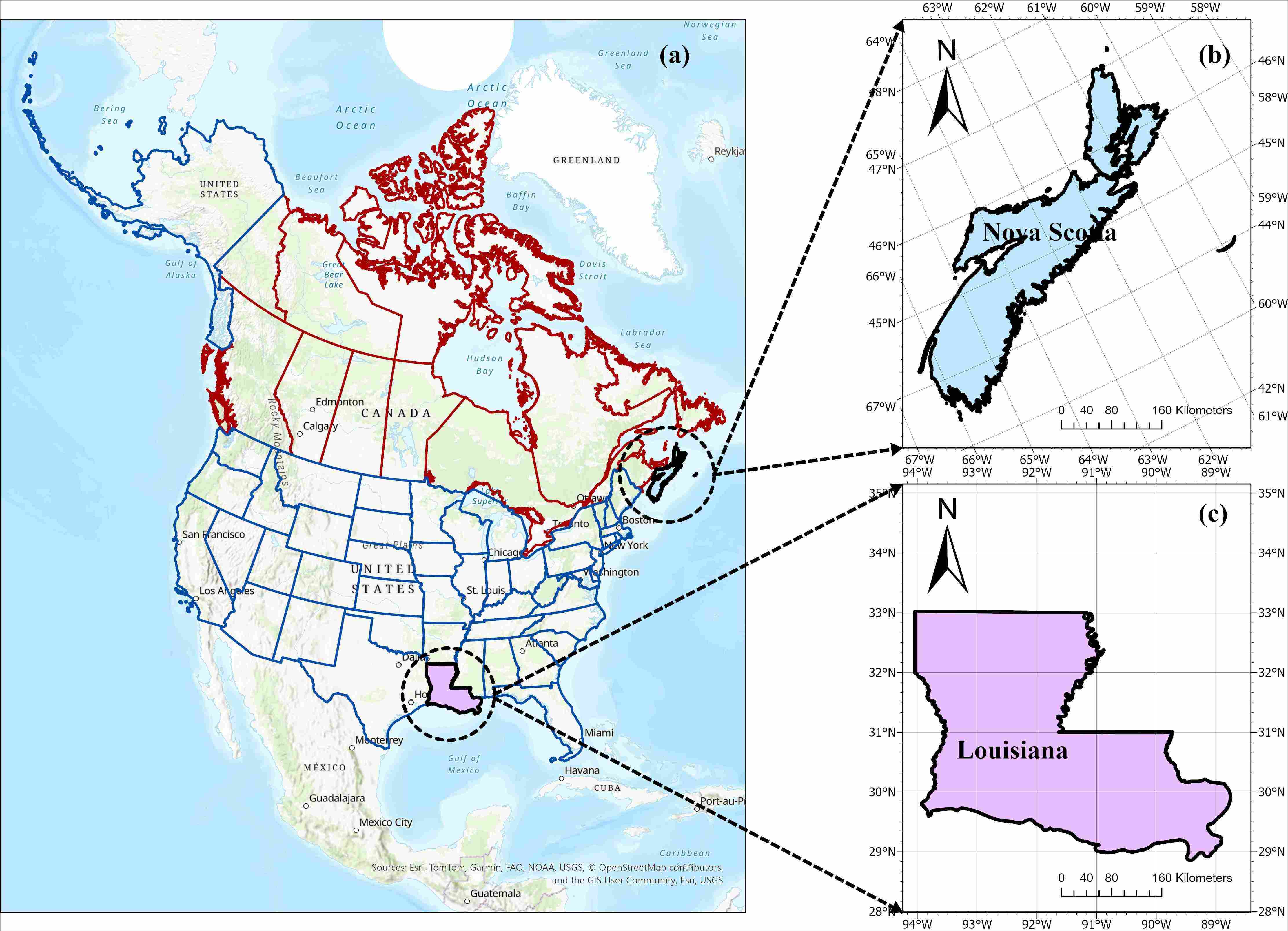 |
2020 | 0.0337 | 0.0325 | ||
2021 | 0.0352 | 0.0326 | ||
2022 | 0.0311 | 0.0303 | ||
2023 | 0.0350 | 0.0320 | ||
2024 | 0.0344 | 0.0336 | ||
NO₂, (mol m⁻²) | 2019 | 6.15×10⁻⁵ | 2.25×10⁻⁵ | |
2020 | 5.80×10⁻⁵ | 2.27×10⁻⁵ | ||
2021 | 6.10×10⁻⁵ | 2.43×10⁻⁵ | ||
2022 | 6.15×10⁻⁵ | 2.54×10⁻⁵ | ||
2023 | 6.36×10⁻⁵ | 2.50×10⁻⁵ | ||
2024 | 5.98×10⁻⁵ | 2.36×10⁻⁵ |
Across 2019–2024, seasonal means of tropospheric column CO exhibit similar phasing in both jurisdictions but domain-dependent magnitudes (Table 2). In NS, seasonal CO means are 0.033441 (winter), 0.03501 (spring), 0.03453 (summer), and 0.03242 mol m⁻² (fall), while LA records 0.03192, 0.03633, 0.02987, and 0.03032 mol m⁻² for the same seasons. Both regions peak in spring, with NS consistently higher than LA in winter, summer, and fall. The standard deviation in NS is largest in summer, indicating greater interannual spread; this pattern reflects, in part, the elevated summer of 2023 and suggests that the NS-LA summer contrast is not strictly stationary across years (NS summer CO coefficient of variation ≈ 10.6%). For NO₂, differences are larger and more stable. NS seasonal means are 4.22×10⁻⁵ (winter), 6.69×10⁻⁵ (spring), 7.54×10⁻⁵ (summer), and 5.94×10⁻⁵ mol m⁻² (fall), compared with LA values of 3.21×10⁻⁵, 2.01×10⁻⁵, 2.09×10⁻⁵, and 2.29×10⁻⁵ mol m⁻². The NS/LA ratio is ~1.3 in winter but rises to ~2.6–3.6 in the warm seasons. Small seasonal standard deviations relative to the means in both domains indicate that these contrasts recur across years rather than being driven by single-year anomalies.
Monthly trajectories refine the seasonal picture by pinpointing diagnostic months and anomalies (Figure 2). In NS (Figure 2a), CO exhibits recurrent late-spring/early-summer crests with a pronounced surge in August 2023 (record monthly high) and a trough in October 2022 (record monthly low). LA shows repeat April maxima, with the highest monthly CO in April 2020, and sustained August minima, including a record low in August 2022. These month-specific peaks and nadirs delineate calendar-aware inspection windows (e.g., NS late spring-summer; LA early spring), enabling like-for-like year comparisons and targeted advisories keyed to expected monthly envelopes rather than broad seasons. The month-level evolution of NO₂ (Figure 2b) highlights systematic phase offsets between the two jurisdictions. NS concentrates its highest monthly NO₂ in July 2023, with recurrent late-winter plateaus near the annual minima (e.g., January 2021, January 2024). LA, by contrast, places its strongest monthly NO₂ in January 2023 and exhibits repeat late-spring minima (e.g., May 2024).
Pollutant | Year | Season | |||||||
Nova Scotia (NS) | Louisiana (LA) | ||||||||
Winter | Spring | Summer | Fall | Winter | Spring | Summer | Fall | ||
CO (mol/m2) | 2019 | 0.034049 | 0.036401 | 0.033551 | 0.030831 | 0.031595 | 0.03696 | 0.029153 | 0.029376 |
2020 | 0.033875 | 0.036193 | 0.031100 | 0.033321 | 0.032741 | 0.037205 | 0.029223 | 0.030290 | |
2021 | 0.034546 | 0.035845 | 0.036746 | 0.034053 | 0.033264 | 0.036051 | 0.030626 | 0.031841 | |
2022 | 0.033399 | 0.033583 | 0.029796 | 0.028398 | 0.031395 | 0.03488 | 0.02745 | 0.027744 | |
2023 | 0.030911 | 0.033724 | 0.039144 | 0.03483 | 0.029128 | 0.03507 | 0.030845 | 0.031084 | |
2024 | 0.033867 | 0.034302 | 0.036848 | 0.033055 | 0.033390 | 0.037787 | 0.031894 | 0.031598 | |
Statistics | Winter | Spring | Summer | Fall | Winter | Spring | Summer | Fall | |
Mean | 0.033441 | 0.035008 | 0.034531 | 0.032415 | 0.031919 | 0.036325 | 0.029865 | 0.030322 | |
StD | 0.001293 | 0.001282 | 0.003653 | 0.002383 | 0.001601 | 0.001188 | 0.001575 | 0.001553 | |
NO₂ (mol/m2) | 2019 | 4.79×10⁻⁵ | 7.04×10⁻⁵ | 7.64×10⁻⁵ | 5.68×10⁻⁵ | 2.85×10⁻⁵ | 1.98×10⁻⁵ | 1.87×10⁻⁵ | 2.16×10⁻⁵ |
2020 | 3.71×10⁻⁵ | 6.41×10⁻⁵ | 7.17×10⁻⁵ | 5.62×10⁻⁵ | 3.20×10⁻⁵ | 1.77×10⁻⁵ | 2.02×10⁻⁵ | 2.02×10⁻⁵ | |
2021 | 3.82×10⁻⁵ | 6.66×10⁻⁵ | 7.68×10⁻⁵ | 6.08×10⁻⁵ | 3.22×10⁻⁵ | 1.97×10⁻⁵ | 2.27×10⁻⁵ | 2.38×10⁻⁵ | |
2022 | 4.51×10⁻⁵ | 6.54×10⁻⁵ | 7.35×10⁻⁵ | 6.03×10⁻⁵ | 3.26×10⁻⁵ | 2.23×10⁻⁵ | 2.26×10⁻⁵ | 2.53×10⁻⁵ | |
2023 | 4.57×10⁻⁵ | 7.06×10⁻⁵ | 7.93×10⁻⁵ | 6.49×10⁻⁵ | 3.23×10⁻⁵ | 2.12×10⁻⁵ | 2.01×10⁻⁵ | 2.35×10⁻⁵ | |
2024 | 3.97×10⁻⁵ | 6.40×10⁻⁵ | 7.44×10⁻⁵ | 5.76×10⁻⁵ | 3.49×10⁻⁵ | 1.96×10⁻⁵ | 2.09×10⁻⁵ | 2.32×10⁻⁵ | |
Statistics | Winter | Spring | Summer | Fall | Winter | Spring | Summer | Fall | |
Mean | 4.22×10⁻⁵ | 6.69×10⁻⁵ | 7.54×10⁻⁵ | 5.94×10⁻⁵ | 3.21×10⁻⁵ | 2.01×10⁻⁵ | 2.09×10⁻⁵ | 2.29×10⁻⁵ | |
StD | 4.50×10⁻⁵ | 2.98×10⁻⁵ | 2.70×10⁻⁵ | 3.26×10⁻⁵ | 2.05×10⁻⁵ | 1.57×10⁻⁵ | 1.56×10⁻⁵ | 1.79×10⁻⁶ | |
The Sentinel-5P-derived CO and NO₂ concentration raster files shown in Figures 3 and 4 illustrate the spatial distribution of column concentrations across NS and LA. Jenks Natural Breaks with five classes was used to highlight hotspots where discrete classification was appropriate, while a continuous colour ramp was applied where the number of unique values made Jenks classification impractical, such as in Figure 3a. To distinguish between concentration values, Jenks with 5 classifications was used to better highlight hot spots, and in other cases, colour ramp was used. A colour gradient was applied when the number of unique values was too high and using Jenks was impractical (Figure 3a), ensuring clear visualisation of CO concentrations. In NS, Very High classes oscillate from 0.0339–0.0352 mol m⁻² (2019), ease in 2022 (≈ 0.0317–0.0328 mol m⁻²), and rebound by 2024 (≈ 0.0351–0.0369 mol m⁻²), with hotspots recurring over the south-western corridor and Halifax-Dartmouth environs and episodically extending eastward. LA shows a broadly upward trajectory punctuated by a 2022 dip; hotspots are frequent over northern parishes and along the Mississippi River industrial/delta belts. Because these are CO column concentrations (mol m⁻²), not emissions, the persistent hotspot geography and year-to-year amplitude shifts are reported as spatial patterns rather than direct evidence of emission changes.
NO₂ maps display pronounced, jurisdiction-specific corridors whose location is stable while magnitudes vary interannually, identifying areas where future ground monitoring and exposure assessment could be prioritised (Figure 4). In NS, High-Very High burdens cluster around the Halifax-Dartmouth axis and North Sydney, whereas Truro-Tatamagouche repeatedly fall in Low classes; a 2019 baseline of 6.521x10⁻⁵–7.494×10⁻⁵ mol m⁻² gives way to broad reductions in 2020 (6.357×10⁻⁵–7.076×10⁻⁵ mol m⁻²). LA exhibits heterogeneous High-Very High hotspots along the Baton Rouge-New Orleans corridor (Mississippi River) with Low classes over many northern/southern parishes; a jurisdictional peak in 2021 (4.429×10⁻⁵–7.221×10⁻⁵ mol m⁻²) is followed by step-down reductions through 2024. The stable NO₂ hotspot locations and variable intensities indicate recurring spatial clustering of elevated NO₂ columns, particularly around the Halifax-Dartmouth and North Sydney areas in NS and the Baton Rouge-New Orleans corridor in LA.
Sentinel-5P provides tropospheric column burdens (mol m⁻²), whereas ground monitors measure near-surface concentrations (e.g., ppb/µg m⁻³). Because these quantities differ in vertical support, chemistry, and sampling, direct regression is not a “validation” and can yield weak or even sign-reversing relationships, especially under stable boundary layers, coastal marine layers, and strong vertical decoupling. Moreover, province/state aggregation smooths subregional gradients and can amplify representativeness mismatch where monitors are clustered in urban/near-road environments. Accordingly, Figure 5 is used as a consistency/representativeness diagnostic, not a product-accuracy test.
Across 2020–2023, NS shows weak CO correspondence with ground data (R² = 0.09; Figure 5a), while LA performs modestly better for CO (R² = 0.37; Figure 5b). For NO₂, NS exhibits stronger concordance but in a negative direction (R² = 0.78; slope = −0.33; Figure 5c), whereas LA’s NO₂ relationship is weaker (R² = 0.26; Figure 5d). Since each regression is based on only four annual observations, the fitted lines, R² values, and slopes are interpreted as descriptive diagnostics only and do not support robust statistical inference or formal validation. These exploratory comparisons are consistent with known column-surface representativeness limits: column retrievals integrate the full tropospheric burden and can vary with mixing depth and vertical profile structure, while surface monitors sample local near-ground air that can be vertically decoupled, particularly in winter stability and marine boundary-layer conditions. Therefore, weak or negative relationships do not imply “large satellite errors”; rather, they delimit how the two observing systems should be combined, satellites to map spatial gradients and identify seasonal timing windows, and surface networks to quantify exposure and evaluate compliance at specific locations. Given the small sample size, Figure 5 is used only as an exploratory consistency check and not as a formal validation of satellite-surface agreement. Future work will extend this diagnostic to monthly/season-stratified comparisons and station-buffered satellite sampling to better match surface network spatial support.
4. Discussion
The results are relevant to sustainability because they show that coastal air-quality management should consider both timing and location. Rather than relying only on annual averages, the observed spring CO peaks in both regions, summer NO₂ peaks in NS, winter NO₂ peaks in LA, and recurring hotspot corridors suggest that monitoring programs can be better aligned with periods and places of higher column burdens. This provides a practical link between satellite-based air-quality monitoring, public health screening, and sustainable coastal governance under SDG 3 and SDG 11. The spatiotemporal patterns of CO and NO₂ columns across NS and LA are consistent with our central interpretation, while not providing direct causal proof of meteorological control. The empirical outcomes are broadly consistent with our expectations, although the seasonal phasing requires a more precise interpretation: CO reaches its highest seasonal mean in spring in both jurisdictions, while NO₂ peaks in summer in NS and winter in LA. The synchronised 2022 CO minimum is treated here as a shared interannual feature rather than evidence of a single confirmed cause. These findings are consistent with a possible role for boundary-layer dynamics and maritime ventilation in shaping coastal pollutant columns, alongside local activity patterns; however, this study does not directly test these mechanisms. The following discussion interprets these confirmed patterns within the context of atmospheric processes and broader literature.
NS and LA annual CO and NO₂ contrasts (Table 1) indicate that column concentrations should not be interpreted from source intensity alone; instead, the observed patterns are consistent with possible influences from geography, seasonal mixing, and coastal meteorological setting. NS’s persistently higher NO₂ columns are consistent with combustion activity and conditions that can concentrate plumes (Gibson et al., 2013; Hoffman et al., 2017; Mitchell et al., 2021). Remote communities relying on diesel generators, such as those in coastal Labrador, exemplify how stationary combustion sources can contribute to local NO₂ burdens, though hybrid renewable systems offer a viable alternative for emissions reduction (Kotian & Ghahremanlou, 2024). LA’s lower, moderately stable NO₂ aligns with humid-subtropical conditions, sea-breeze ventilation (Athul et al., 2025; Avila Rodríguez et al., 2024; Weber, 2023). In short, the two-to-one NO₂ split and tightly ranged CO indicate atmosphere-surface coupling (Blanchard et al., 2019), rather than simple emission totals (Reid & Aherne, 2016). Synchronized interannual features also support this interpretation: the 2020 NO₂ downturn tracks COVID-19 pandemic mobility/operations reductions (Azad & Ghandehari, 2022; Fioletov et al., 2022), the 2022 CO minimum is consistent with economic slowdowns and favorable ventilation (Campbell et al., 2021; Zeng et al., 2022). Elevated 2021/2023 columns cohere with wildfire years and long-range transport that loft and sustain carbon-rich plumes (Ehret et al., 2025), which can sometimes decouple columns from surface monitors (Stevens et al., 2024). These annual means establish a mechanistic baseline for year-over-year evaluation, calibrating policy check-ins to shared nadirs/peaks while interpreting trend direction through mixing and meteorology rather than through emission totals alone.
Although our analysis focuses on concentration patterns rather than explicit meteorological modelling, the seasonal and monthly phasing we observe, in Table 2 and Figure 2, is consistent with established boundary-layer and synoptic regimes in both domains. In NS, frequent marine boundary layers, recurrent nocturnal inversions, and suppressed daytime mixing under cool-maritime influence are expected to reduce effective ventilation; episodic advection of boreal fire plumes further augments warm-season column burdens (Busilacchio et al., 2016; Dadashazar et al., 2021; Lozovatsky et al., 2021). These processes coherently align with the summer-dominated NO₂ and elevated warm-season CO seen in the monthly record, including the 2023 summer crest; intermittent autumn-winter inversions plausibly explain late-year troughs and shoulder-season rebounds without invoking changes in emissions (Mitchell et al., 2021). In LA, the complementary pattern, winter-peaked NO₂ and spring-biased CO maxima, is consistent with cool-season stability, shallower boundary layers, continental northerlies, and reduced photochemical loss rates during winter, followed by transitional meteorology and agricultural-burning signals in spring (Bhattarai et al., 2024; Liu et al., 2016). This phase contrast is consistent with possible differences in coastal stability regimes, while stable NO₂ hotspots may reflect recurring corridor activity and the shared 2022 CO minimum may reflect broader interannual conditions affecting both regions. The persistence of January NO₂ peaks and late-spring minima across multiple years suggests a robust timing signature rather than a single-year anomaly. Pandemic-period activity reductions likely sharpened seasonal contrasts by temporarily depressing traffic- and industry-related precursors, most visibly in spring 2020 NO₂ minima and selective CO anomalies. We treat these as exogenous shocks that accentuate, rather than create, the underlying phasing (Chen et al., 2020; Ghahremanlou & Kubiak, 2023; Zhao et al., 2022). That said, we refrain from causal attribution beyond consistency, as rigorous attribution would require co-modelled covariates (e.g., ERA5 BLH, winds, temperature, fire radiative power) and formal time-series controls (Ghahremanlou & Ghahremanlou, 2025a). From a governance standpoint, the month-specific crests and troughs we identified (e.g., NS mid-summer; LA mid-winter) provide calendar-aware evaluation windows for satellite-ground alignment, hotspot verification, and inspection scheduling. This timing lens can help improve comparability across years and helps avoid misattributing dynamics that are primarily phase driven. In the context of evolving policy, tightening fossil-fuel constraints in NS versus infrastructure expansions and hurricane-mediated variability in LA, calendar-aware monitoring can serve as structural relief, guiding the deployment of ground sensors, episodic advisories, and targeted enforcement (Giacosa et al., 2023; Lee et al., 2022; Maliat et al., 2024; Smith et al., 2025).
In NS, recurrent south-western and Halifax-Dartmouth CO hotspots, High-Very High, in Figure 3 are compatible with maritime boundary layers (Lozovatsky et al., 2021), household heating superimposed on traffic (Brett et al., 2025), while Cape Breton remains comparatively low under stronger offshore ventilation and limited industry (Gibson et al., 2013). In such urban-coastal corridors, Nature-Based Solutions like urban forests and green infrastructure could provide complementary mitigation, as evidenced by satellite-monitored reductions in land surface temperature (≈2.1 °C) and substantial increases in carbon storage following park interventions (Zanardi et al., 2025). In LA, the Mississippi River industrial/delta belt sits where petrochemical emissions meet humid subtropical air masses (Haider et al., 2025), a setting that is consistent with photochemical processing and corridor accumulation (Robinson et al., 2024). Similarly, Alberta’s enhancements tied to oil-sands activity and weak ventilation contrast with California’s COVID-era declines, underscoring CO’s responsiveness to activity and mixing (Liu et al., 2021; Marey et al., 2015); globally, peaks over the Indo-Gangetic Plain, in Wuhan (China), and in Makassar (Indonesia) reinforce the primacy of source type (Dhankar et al., 2024; Liu et al., 2025; Makhsud & Sulistyono, 2018). Practically, these column maps can help guide place-based audits along ports, petrochemical belts, and arterial corridors and support time-aware advisories aligned to known ventilation regimes (Xiong et al., 2022) and urban growth patterns (Behera et al., 2025; Mohan et al., 2025).
In NS (Figure 4), the Halifax-Dartmouth and North Sydney axes sit at the confluence of Atlantic maritime inflow and continental outflow, fostering persistent NO₂ accumulation zones even when local activity fluctuates (Athul et al., 2025; Dadashazar et al., 2021). In LA, the Baton Rouge-New Orleans Mississippi River corridor functions as a “thermal highway”, where industrial heat islands and humid subtropical air masses promote convective recirculation and patchy, high-intensity plumes (Tzavali et al., 2015), a dynamic consistent with the 2021 peak followed by step-down reductions (Mitchell et al., 2021). Such persistent urban NO₂ accumulation patterns align with findings from other metropolitan regions, where satellite-derived clustering analysis has identified High-High concentration zones that remain stable across seasons despite variable meteorological conditions (Ghahremanlou & Ghahremanlou, 2025a). This interpretation is kept focused on the NS-LA contrast: differing coastal stability helps explain the summer NO₂ peak in NS and winter NO₂ peak in LA, while fixed corridor activity helps explain stable NO₂ hotspots and broader interannual conditions likely explain the shared 2022 CO minimum. Pollution exposure may be shaped not only by spatial patterns but by the rhythms of urban life, which can contribute to uneven air-quality burdens across communities (Singh et al., 2025; Walker et al., 2022). The stable NO₂ locations but variable magnitudes support corridor-specific controls (Enuneku et al., 2024), future equity-aware network planning where appropriate demographic or vulnerability data are available, and calendar-timed inspections when columns predictably rise, supporting targeted NO₂ management (Xu et al., 2020).
Our 2020–2023 regressions in Figure 5 treat satellite columns as consistency checks, not flux equivalence, and the outcomes map known jurisdictional sensitivities (unit and domain differences) (Ukhov et al., 2020). While this province/state-scale approach yields interpretable jurisdictional contrasts, it inevitably smooths subregional variability and does not fully resolve the representativeness and sampling-mismatch issues inherent in satellite-surface comparisons. Column retrievals integrate the total tropospheric burden, whereas surface monitors sample near-ground air that can be vertically decoupled under stable boundary layers, particularly in winter (Xiang et al., 2019). The resulting weak or even negative correlations therefore reflect physical disconnects rather than methodological error. In LA, moderate CO/NO₂ agreement reflects spatially aggregated petrochemical corridors where column footprints and ground siting overlap more coherently (Thompson et al., 2023), whereas in NS, stronger NO₂ but weak CO correspondence is plausible over diffuse coastlines with marine ventilation and vertical decoupling that reduce column-surface coherence (Jalali et al., 2022). Winter stratification can also degrade correlations by disconnecting near-surface loadings from total columns (Rodionova, 2022). Cross-regional evidence is consistent, southern African wintertime stratification led to satellite overestimation at the surface (Ngcoliso et al., 2025); and in the Pearl River Delta and Colombian cities, NO₂ aligned better than CO due to urban-rural gradients and hotspot aggregation (Barten et al., 2020; Hu et al., 2021). Gaps in long-term assessments of NO₂ exposure effects, particularly in vulnerable populations, remain a key concern, including evidence of high episodic exposure in parks (Simón-Moral et al., 2025). These gaps reinforce the continued need for consistent, high-resolution monitoring, and hybrid monitoring approaches that integrate satellites, ground networks, and meteorology (Bendib & Boutrid, 2024; Ngo et al., 2021). Such approaches should also account for local boundary-layer regimes and platform limitations to turn consistency signals into defensible policy actions (Ghahremanlou & Ghahremanlou, 2025b; Seo et al., 2025).
Satellite column concentrations from Sentinel-5P help identify when and where column burdens rise in NS and LA, suggesting that governance could move beyond static, inventory-centric checks toward calendar-aware, corridor-specific oversight. In NS, publish summer evaluation windows (wildfire/photochemical season) and pair them with transport/port audits, surge smoke alerts, and temporary traffic/port operations management; in LA, schedule winter NO₂ audits and strengthen permit conditions for the Mississippi River corridor under stable cold-season layers, with contingency triggers for stagnation episodes. To make monitoring defensible, adopt a regionalized calibration workflow: routine season-specific bias checks, plume-height flags, and satellite-ground fusion (columns to triage hotspots and timing; ground to quantify exposure/compliance). For networks, future monitoring could prioritise equity-focused siting, including rural and Indigenous communities in NS and fenceline or port-adjacent neighbourhoods in LA; however, because this study did not include demographic, income, race, or health-vulnerability layers, these equity references are presented as monitoring recommendations rather than empirical social-vulnerability findings. Regulatory instruments should codify published evaluation calendars, corridor-based inspections, and place-based performance metrics rather than only area-wide annual means, aligning practice with Canada’s Air Quality Management System and US National Ambient Air Quality Standards while acknowledging that concentrations ≠ emissions. Internationally, the Sentinel-5P-observed decline in CO during 2022, coinciding with global economic retrenchment, demonstrates its ability to track concentration responses to macrolevels, aligning with the Paris Agreement’s monitoring needs. Finally, embed adaptive management: pre-authorised seasonal measures (e.g., clean fuel/operations curtailment during forecasted stagnation), rapid post-event reviews (wildfire/hurricane), and transparent data releases to support investigations. Incorporate Sentinel-5P to target hotspots, time inspections to seasonal peaks, and verify outcomes with ground data, so actions are timely, targeted, and climate-resilient. These practical monitoring and policy actions are summarised by jurisdiction, pollutant, season, and hotspot corridor in Table 3.
Jurisdiction | Pollutant | Season | Corridor/Hotspot | Recommended Action |
Nova Scotia (NS) | NO₂ | Summer | Halifax-Dartmouth and North Sydney | Increase summer satellite-ground checks and hotspot verification |
Nova Scotia | CO | Spring | Southwestern corridor and Halifax-Dartmouth area | Review spring CO patterns and coordinate with smoke/event advisories |
Louisiana (LA) | NO₂ | Winter | Baton Rouge-New Orleans corridor | Prioritise winter corridor checks and review monitoring coverage along the Mississippi River industrial corridor |
Louisiana | CO | Spring | Northern parishes and Mississippi River/delta belt | Track spring CO increases and compare satellite patterns with ground networks |
5. Conclusions
This study used Sentinel-5P satellite data to assess multi-year CO and NO₂ trends over NS and LA during 2019-2024 to characterise jurisdiction-scale column dynamics in two contrasting coastal locations. This closed the existing research gap in an innovative dual-pollutant, jurisdiction-scale coastal analysis via a transparent Sentinel-5P workflow with coastal-process interpretation and consistency checks against inventories and ground networks. Across these contrasting regimes, the signal is structural: CO columns are narrowly banded in both jurisdictions (NS 0.0311-0.0352; LA 0.0303-0.0336 mol m⁻²) with a shared 2022 nadir, while NO₂ maintains a stable ≈2.5 split (NS 5.80×10⁻⁵–6.36×10⁻⁵ vs. LA 2.25×10⁻⁵–2.54×10⁻⁵ mol m⁻²). This pattern, tight CO with synchronised minima and persistent NO₂ separation, is consistent with the influence of domain-wide ventilation and boundary-layer processes, but direct meteorological attribution was not performed. The main seasonal result is that CO peaks in spring in both jurisdictions, while NO₂ peaks in summer in NS and winter in LA. Recurring spatial corridors, including Halifax-Dartmouth and Baton Rouge-New Orleans, further indicate where column burdens remain persistent across years.
This study is constrained by its reliance on column concentrations without explicit source separation. Distinguishing anthropogenic from natural contributions would require an inversion framework that links inventories, chemistry, and transport. Resolution and sampling mismatches also persist between Sentinel-5P footprints, sub-grid emitters, and point monitors, as do sensitivities to QA screening and year-specific map legends. Future work should remain focused on three priorities: extending the time series, adding meteorological covariates such as boundary-layer height and wind fields, and improving satellite-surface comparison through monthly or station-buffered sampling.
The satellite evidence here is best used for operational targeting rather than flux attribution. Sentinel-5P columns identify recurring CO and NO₂ hotspots, seasonal evaluation windows, and jurisdiction-specific regimes that support policy design and monitoring. Calendar-aware scheduling aligned with the observed seasonal windows, spring CO in both jurisdictions, summer NO₂ in NS, and winter NO₂ in LA, together with corridor-focused checks in persistent hotspots such as Halifax-Dartmouth and Baton Rouge-New Orleans, can improve monitoring timing and representativeness. Future equity-aware network densification at these corridors, paired with routine satellite-ground consistency checks, could use columns for timing/triage and surface networks for magnitude/compliance, while recognising that demographic and health-vulnerability overlays were not included in this study. Embedding these practices into regulatory workflows, via pre-authorised, time-limited measures triggered by forecasted stagnation, rapid post-event evaluations (wildfire/hurricane), and transparent publication of QA coverage, valid-pixel counts, and class breaks with each map, yields an auditable, adaptive system that shifts regulations from reactive to evidence-timed. Overall, the main sustainability message is that satellite column data can help shift coastal air-quality governance from broad annual review toward more targeted, seasonal, and evidence-timed monitoring.
Conceptualization, A.G., D.G., and S.L.; methodology, A.G., D.G., and S.L.; software, A.G. and D.G.; validation, S.L. and D.G.; formal analysis, S.L. and D.G.; investigation, D.G., A.G., and S.L.; resources, D.G.; data curation, D.G. and S.L.; writing—original draft preparation, S.L. and J.Y.; writing—review and editing, S.L., J.Y., D.G., and A.G.; visualization, S.L., D.G., and A.G.; supervision, D.G.; project administration, D.G. All authors have read and agreed to the published version of the manuscript.
The Google Earth Engine JavaScript scripts, Python analysis scripts, fixed processing parameters, and representative output templates used to support this study are publicly available at: https://doi.org/10.5281/zenodo.20448867. The repository includes scripts for Sentinel-5P CO and NO₂ monthly/annual extraction over NS and LA, annual raster export for GIS-based mapping, Python scripts for annual/seasonal summaries, monthly maximum/minimum diagnostics, monthly trajectory plots, and satellite-surface consistency checks. Sentinel-5P data are publicly available through the Google Earth Engine Copernicus Sentinel-5P collections, and the ground-monitoring/inventory sources are publicly available from the national agencies cited in the manuscript. Derived tables and figures can be regenerated using the fixed parameters documented in the repository.
The authors declare no conflict of interest.